Travelling Salesman Problem

Problem definition

Consider a salesman needing to travel to n cities:

• He can start from any city
• He needs to visit any city once and only once

What is the path with the shortest traveling distance?

This is the TSP: Traveling Salesman Problem

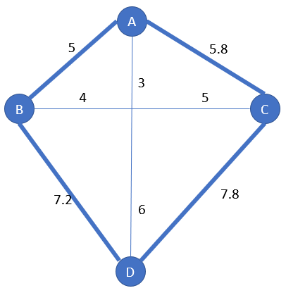
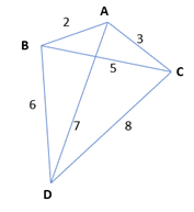
Example with 4 cities:

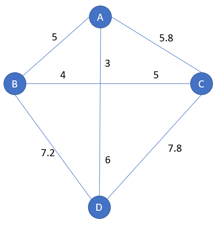
Symmetry / Asymmetry

Above the distance is symmetric: from A to B the distance is the same as B to A, this is named sTSP. By default, the TSP is considered sTSP.

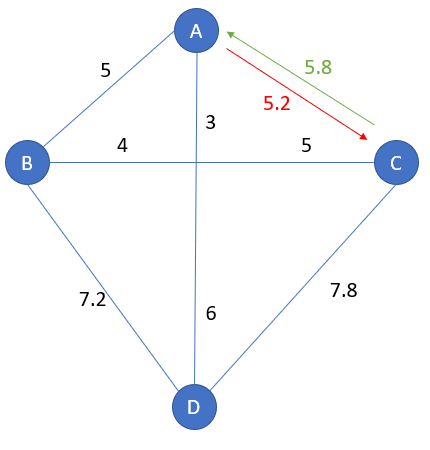
TSP can also consider asymmetric distances, called aTSP. For example, the road isn’t the same between going and coming

Example of an aTSP problem:

How many paths possibles in a TSP?

A naive counting

It can be counted this way:

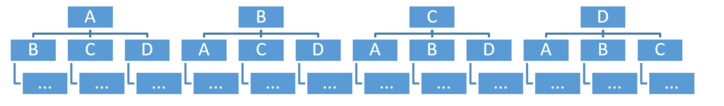
• At the first level: all cities are possible: n possibilities
• At second level: n-1 possibilities (because it is forbidden to visit twice a city)
• …
• At the last level: 1 possibility

For example, the first two levels of a 4-cities problem:

This mean n*(n-1)*(n-2)*…*1 possible paths:

There are n! possible paths

With 4-cities, we can list the 4! = 4*3*2*1 = 24 possibilities

A	B	C	D
B	A	C	D
C	A	B	D
A	C	B	D
B	C	A	D
C	B	A	D
C	B	D	A
B	C	D	A
D	C	B	A
C	D	B	A
B	D	C	A
D	B	C	A
D	A	C	B
A	D	C	B
C	D	A	B
D	C	A	B
A	C	D	B
C	A	D	B
B	A	D	C
A	B	D	C
D	B	A	C
B	D	A	C
A	D	B	C
D	A	B	C

First skimming

If you shift a path, from 1, 2,…,n offset, the distance is same.

For example, the distance of path [A-B-C-D] is the same as [B-C-D-A], and the same as [C-D-A-B] and [D-A-B-C]. Concretely, it means it means is possible to start from a single chosen city.

From the naive count n!, we can divide by n: the first skimming solution is (n-1)! possible paths.

With 4-cities, we can summarize the 24 solutions as solutions starting from the city A, there are 3! = 3*2*1 = 6 solutions. Here we choose to start only from the city A

A	B	C	D
A	C	B	D
A	D	B	C
A	B	D	C
A	C	D	B
A	D	C	B

Last skimming

When the distances are symmetric, when you reverse a path, the distance is the same.

For example, the distance [A-B-C-D] is the same as [D-C-B-A].

With 4-cities, we skim the inverse duplicates:

• Row 1 and 6: row A is [A-B-C-D], its reverse is [D-C-B-A], and after rearrangement, it is similar to [A-D-C-B]
• Row 2 and 3
• Row 4 and 5

There are now 3 solutions:

A	B	C	D
A	C	B	D
A	B	D	C

Final count

If there are n cities, in a symmetric scenario, the total number of paths to evaluate is (n-1)!/2

How difficult is it to solve the Traveler Salesman Problem?

There is no problem with the calculation of distances: this is basically additions.

There is an issue with the number of distances to calculate, due to the factorial effect:

Number of cities	Number of solutions
4	3
10	181440
20	6.0823E+16
30	4.4209E+30
40	1.0199E+46
50	3.0414E+62
60	6.9342E+79
70	8.5561E+97
80	4.473E+116
90	8.254E+135
100	4.666E+155

Already with 20 cities, there are around 40.000.000.000.000.000 paths to calculate.

With 100 cities, surely your desktop or laptop won’t finish the calculations before the end of the XXIst century.

Specificity of the TSP

Despite the aim is to find the shortest path, if there are too many cities, the aim will be to find the best possible short path! It may not be the shortest one, indeed no possibility of checking it.

Hence, the idea if to try several algorithms, compare them, and choose the one with the minimum distance.

Algorithm for solving the TSP

Nearest insertion algorithm example

Algorithm definition

• Starting step
• Choose a starting city I
• Find a new city R such that the distance R-I is minimal. The starting subpath is [I-R-I]
• Regular step
• Selection step: find the city R closest to any city of the current subpath, meaning finding the city R, such that for any city J in the subpath, the distance(R-J) is minimal
• Insertion step: from the current subpath, find the adjacent cities I and J, where R has a minimal cost of insertion distance(I-R) + distance(R-J) – distance(I-J). Insert R between I and J
• If the travel is complete, stop, else go to regular step

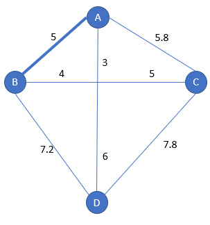
Example with 4 cities

1 – Starting step

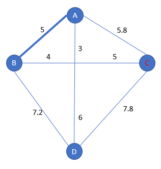
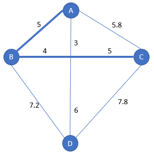
We start from city A.

We choose the nearest city from A: it is B with a distance of 5:

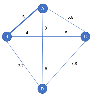
Hence the starting subpath is [A-B-A]

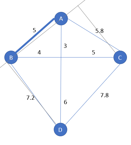
2 – Regular step

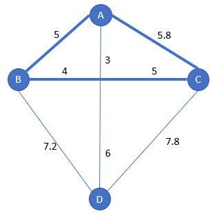
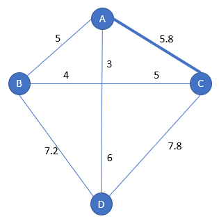
We choose the nearest city from the subpath [A-B-A]: this is C with a distance of 5.8 from A:

For the insertion of C into [A-B-A], it could be:

• [A-C-B-A]
• [A-B-C-A]

Let’s compare the minimal insertion cost:

• [A-C-B-A]: distance(A-C) + distance(C-B) – distance(A-B) = 5.8 + 9 – 5 = 9.8
• [A-B-C-A]: distance(B-C) + distance(C-A) – distance(A-B) = 9 + 5.8 – 5 = 9.8

Have you noted the distance is the same? It’s because, in this step, we have basically a triangle, with symmetric distances, hence the paths are the same.

The subpath [A-B-C-A] is chosen amongst the two (quite the same) possibilities.

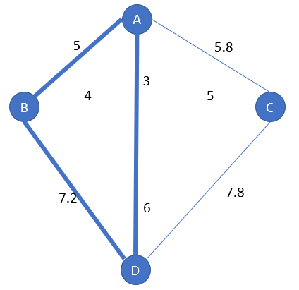
3 – Regular step

It remains one city to select, so finding the city with the closest distance to any city of the current subpath is easy

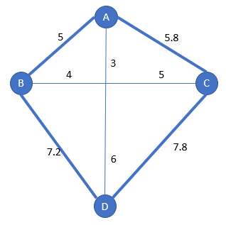
It remains one city D to insert:

• [A-D-B-C-A]
• [A-B-D-C-A]
• [A-B-C-D-A]

Amongst these 2 options, which one minimizes the insertion distance?

• [A-D-B-C-A] has an insertion distance of distance(A-D) + distance(D-B) – distance(A-B) = 9 + 7.2 – 5 = 11.2
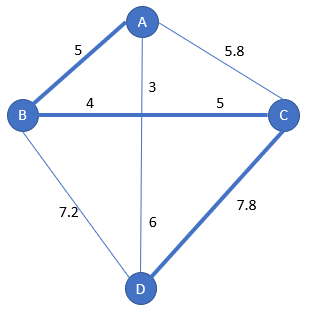
• [A-B-D-C-A] has an insertion distance of distance(B-D) + distance(D-C) – distance(B-C) = 7.2 + 7.8 – 9 = 6
• [A-B-C-D-A] has an insertion distance of distance(C-D) + distance(D-A) – distance(C-A) =7.8 + 9 – 5.8 =11

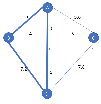
The winner with the nearest insertion step is [A-B-D-C-A] The total distance from this algorithm is 20.

Performance of the algorithm

A scholarly and complex calculation indicates that the distance with the nearest insertion is no more than twice the optimal distance.

The number of required calculations is increasing with the square of n: conventionally written as O(n²)

Cheapest insertion algorithm

Algorithm definition:

The cheapest insertion is the cousin of the nearest insertion. The nearest insertion is looking for the closest city, and then is looking for the minimal insertion cost.

The cheapest insertion is more accurate, and thus requires more calculation: every city is a candidate (instead of the closest city), and then every minimal insertion cost is checked.

This means the cheapest insertion:

• is as good or better than nearest insertion
• requires more calculations

The steps of the cheapest insertion algorithm:

• Starting step
• Choose a starting city I
• Regular step
• From the current subpath, find the city R, not in the subpath, and two adjacent cities in the subpath I and J, such that the cost of insertion is minimal: meaning distance(I-R) + distance(R-J) – distance(I-J)
• If the travel is complete, stop, else go to regular step

Example with 4 cities

Step 1

We start from city A.

We look for the city X such as distance A-X-A is minimum (the step is the same as nearest insertion):

• with A-B-A the distance is 5+5=10
• with A-C-A the distance is 5.8+5.8=10.6
• with A-D-A the distance is 9+9=18

C procures the cheapest insertion and is selected:

Step 2

Now we are looking between B and D which one procures the cheapest insertion inside the subpath [A-C-A]:

• for insertion of B, we have the options [A-B-C-A] and [A-C-B-A]
• for insertion of D, we have the options [A-D-C-A] and [A-C-D-A]

The insertion costs are:

• [A-B-C-A]: distance(A-B) + distance(B-C) – distance(A-C) = 5 + 9 – 5.8 = 8.2
• [A-C-B-A]: distance(C-B) + distance(B-A) – distance(C-A) = 9 + 5 5.8 = 8.2
• [A-D-C-A]: distance(A-D) + distance(D-C) – distance(A-C) = 9 + 7.8 – 5.8 = 11
• [A-C-D-A]: distance(C-D) + distance(D-A) – distance(C-A) = 7.8 + 9 – 5.8 = 11

You have noted, like for nearest insertion, some ways are redundant: it is like to the symmetryc distance and triangle effect.

[A-B-C-A] and [A-C-B-A] are the winners, and arbitrarily, [A-B-C-A] is the chosen one.

Step 3

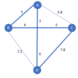
It remains the city D to insert in the subpath [A-B-C-A], the options are:

• [A-D-B-C-A]
• [A-B-D-C-A]
• [A-B-C-D-A]

The insertion costs are:

• [A-D-B-C-A]: distance(A-D) + distance(D-B) – distance(A-B) = 9 + 7.2 – 5 = 11.2
• [A-B-D-C-A]: distance(B-D) + distance(D-C) – distance(B-C) = 7.2 + 7.8 – 9 = 6
• [A-B-C-D-A]: distance(C-D) + distance(D-A) – distance(C-A) = 7.8 + 9 – 5.8 = 11

The calculations provide [A-B-D-C-A] as the winner:

Performance of the algorithm

A sophisticated calculation indicates that the distance with the nearest insertion is no more than twice the optimal distance.

The number of required calculations is increasing with the square of n²*log(n): conventionally written as O(n².log(n))

Nearest Neighbor Algorithm

Algorithm definition:

This algorithm is easier than the precedent ones: the aim is to find the closest city and to add it at the end of the subpath, without looking for a better insertion cost inside the subpath.

As consequences, Nearest Neighbour:

• is less performant than the previous algorithm
• unintuitively, it doesn’t reduce so much the number of calculations compared to nearest insertion

The steps of the nearest neighbor algorithm:

• Starting step
• Choose a starting city
• Regular step
• From the current subpath, find the city R which is the closest to the last city of the current subpath. Add this city R to the end of the subpath.
• If the travel is complete, stop, else go to regular step

Example with 4 cities

Step 1

We start from city A.

Step 2

We choose the nearest city from A: it is B with a distance of 5:

Hence the starting subpath is [A-B-A]

Step 3

We choose the nearest city from the last city of [A-B], which is indeed B.

And the closest city from B is D. The current subpath is [A-B-C]:

Step 4

It remains only one city, D, which is added at the end of the current subpath.

The solution from the algorithm is [A-B-C-D].

It’s better to include the start city, so we can compare with the previous solutions, which provides [A-B-C-D-A]

Performance of the algorithm

A scholarly and complex calculation indicates that the distance with the nearest insertion is no more than 0.5 * rounded_to_upper_integer[log₂(n)] + 0.5

The number of required calculations is increasing with the square of n²: conventionally written as O(n²)

Farthest insertion

Algorithm description

This algorithm is more visual than the others, it requires to draw lines and to estimate distances between points and lines.

The steps are:

• Starting step
• Find the two cities I and J with the farthest distance. Draw an edge between I and J.
• The city R to be added is the one which is the farthest from the edge[I-J]
• Regular step
• From all the edges of the subpath, chose the city R with the maximal distance.
• Find the closest edge [I-J] of the subpath from city R
• Replace this edge [I-J] by the two edges [I-R] and [R-J]

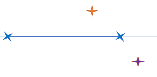
Reminder: how to calculate the distance to and edge

For the orange and violet point, we are looking the distance from the edge of the two blue points:

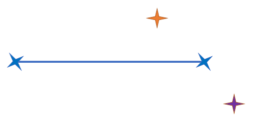
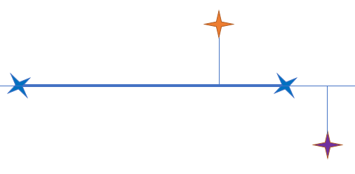
We transform the edge into a line:

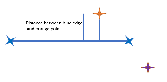
We draw the perpendiculars to the line:

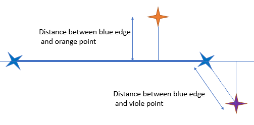
The perpendicular of the orange point is touching the edge: its distance is the one between the blue edge and the orange point

The perpendicular of the violet point is not touching the edge: its distance is the one between the violet point and the closest blue point.

Example with 4 cities

We start with cities A and B which have the smallest distance:

Between C and D, D has the farthest distance from the edge [A-B]:

Hence, the subpath [A-B] is replaced by [A-D-B]:

Now it remains only one city, C.

Its minimal distance to the tour is designated hereunder:

So, the subpath[A-D] is replaced by the subpath [A-C-D]:

The solution is [A-B-D-C]

Concorde code

Definition of the underlying algorithm

It’s very complex to understand. The main parts of the algorithm:

• It finds a very good initial path with an algorithm called Chained Lin-Kernighan
• It improves this initial path with Branch-and-Bound, Branch-and-Cut algorithm and solver.

It is only for symmetric distance. It’s the best solver as it often provides a perfect solution.

Feel free to provide me vulgarized information about its methodology;

Areas of applications

The Concorde solver can be used only for educational purposes.

You cannot use it in a commercial way, for your company or your customer!

Concorde implementation

The main site is: http://www.math.uwaterloo.ca/tsp/concorde/index.html

You can download the Concorde code at http://www.math.uwaterloo.ca/tsp/concorde/downloads/downloads.htm

And you’ll be able to call this solver from the TSP R-library

It’s also possible to work with Concorde solver as a stand-alone.

Windows users, please note that you’ll need to install Cygwin too : https://www.cygwin.com/

Handling Concorde

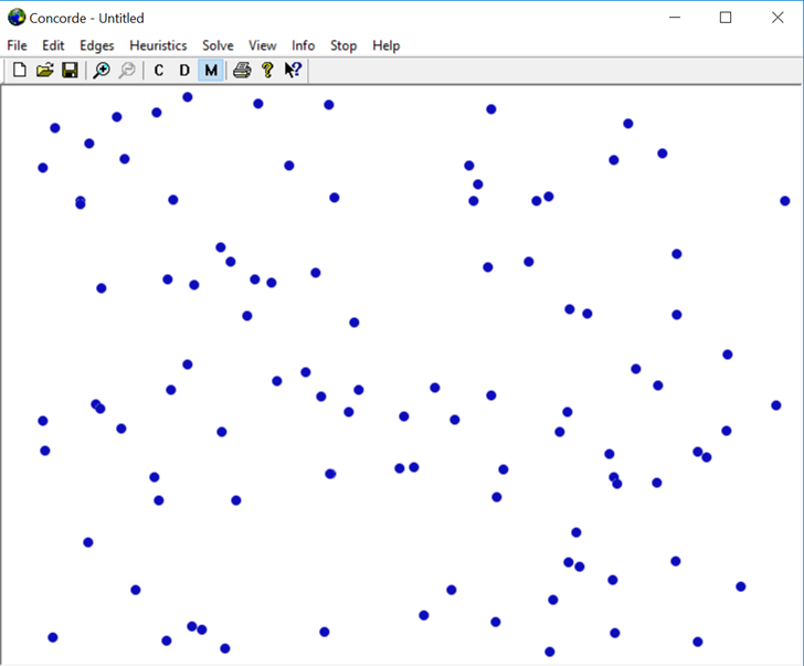
When Concorde GUI is installed, you can, for example, generate some random nodes :

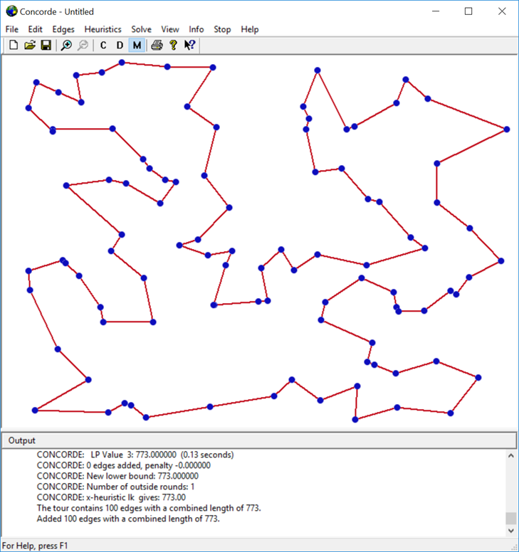
And then run the solver :

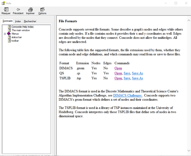
You also can load some configuration file containing your own cities, in a relevant file format :

Application with language R to a 4-cities example 

This link https://vgir.fr/toolbox/ provides information about R installation.

We will use the TSP library, and precise we want to apply the Nearest Insertion Algorithm

We need to manually create a matrix of all distances:

Tips:

• The distance between A and A is not relevant, no need to fill the matrix
• Here we have symmetric distances, hence the matrix is symmetric
• You read the matrix « from / to »  as « row /to column »

We note the distances:

Distance from/to	A	B	C	D
A	–	2	3	7
B	2	–	5	6
C	3	5	–	8
D	7	6	8	–

Please note that TSP library will translate cities into numbers, as numbers are consistent with row and column numbers

A	1
B	2
C	3
D	4

Hereunder the code for creation of the matrix:

# call the TSP library
library(TSP)
# manually create the lines of the matrix
matrix_row1 <- c(0,2,3,7)
matrix_row2 <- c(2,0,5,6)
matrix_row3 <- c(3,5,0,8)
matrix_row4 <- c(7,6,8,0)
# bind the vector row by row
matrix <- data.matrix(rbind(matrix_row1, matrix_row2,matrix_row3,matrix_row4))
# Note that a matrix m is only symmetric if its rownames and colnames are identical. Consider using unname(m). 
rownames(matrix) <- NULL
# adapt the format to the one required by the library TSP                      
tsp_matrix <-  as.TSP(matrix)

The matrix matrix is created:

     [,1] [,2] [,3] [,4]
[1,]    0    2    3    7
[2,]    2    0    5    6
[3,]    3    5    0    8
[4,]    7    6    8    0

We call the solver. Please note in the manual all the available algorithms https://cran.r-project.org/web/packages/TSP/TSP.pdf :

tour <- solve_TSP(tsp_matrix, method = "nearest_insertion")
tour

The result is:

object of class ‘TOUR’ 
result of method ‘nearest_insertion’ for 4 cities
tour length: 19 

So, the minimal distance is 19 with the Nearest Insertion Algorithm.

We ask the corresponding path:

tour_solution <- as.vector(tour)
tour_solution

Manually we can convert this list: the solution 1 2 4 3 is converted as A B D C.

Which tools for solving a TSP?

As described above, you cannot use the Concorde solver in a non-environment.

Hence, it’s forbidden at your job, as an employee, as a consultant.

Run all the possible algorithms available in your language/library, and keep the best one.

Consider using another language, if it contains a promising library

Type of distance / Context	Educational	Business, Consulting,…
Symmetric distances	Concorde: Optimal solution	TSP libraries Consider licensed software   Suboptimal solution
Asymmetric distance	Compare: TSP open-source libraries Concorde by approximation  from  aTSP to tTSP   suboptimal solution	TSP libraries   Suboptimal solution