Introduction

The aim is to answer the question:

Are genetic algorithms inspired by genes?

We’ll compare the original tools of nature with the corresponding tools of genetic algorithms, in order to argue.

Meanwhile, it will lead to a description of the basic concepts of genetic algorithms.

Each genetic algorithm tool will be explored in a 3-steps process:

• How is it in nature?
• How is it adapted to the Travelling Salesman Problem (TSP) as a working scenario?
• An application with a straightforward example of TSP – optional.

---

Choice of a TSP application

We’ll work with the Travelling Salesman Problem (TSP).

It is a relevant scenario for comparison and understanding with Genetic Algorithm.

The TSP concept has already been explained in a previous post: https://vgir.fr/2020/03/01/travelling-salesman-problem-tsp-concept/

The example is slightly modified from the above post, to be more precise and to compare it later with a Python program:

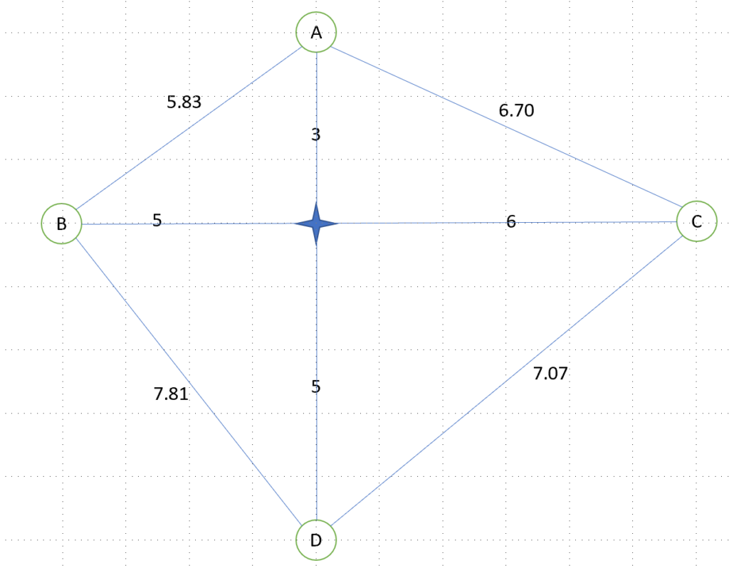
A reminder of the TSP example – the aim is for a Salesman to:

• Visit all the cities A, B, C, D
• Start with city A
• Visit any city once and only once
• Loop the trip and go back to city A at the end
• Find the shortest path, as the Salesman’s time is valuable

---

A quick reminder of genes in nature

In summary, the cells of plants animals, and many other living beings contain a nucleus.

This nucleus contains chromosome(s).

One chromosome is a DNA (Deoxyribonucleic acid) molecule, structured as a long double helix.

The DNA molecule, through its sequence, contains genetic information.

These 2 helixes of DNA are complementary: despite they are not the same, from one you can guess the other. In other words, only one helix is enough to store the information.

Living beings using DNA also use RNA (Ribonucleic acid): in short, keeping only one DNA helix, this becomes RNA, which is a temporary support. Its role is to catalyze biological reactions, control gene expression, and sense and communicate responses to cellular signals.

Focus on the colors: at each « step » of the sequence of the RNA, four different molecules can be present:

• Cytosine – C
• Guanine – G
• Adenine – A
• Uracil – U

The sequence of these molecules is a medium for genetic information.

About writing norms, our example of Uracil then Cytosine then Adenine then Guanine then Uracil sequence will be written in this blog as U-C-A-G-U

---

Application of genes to Travelling Salesman Problem (TSP)

We will write all our paths similarly to an RNA sequence.

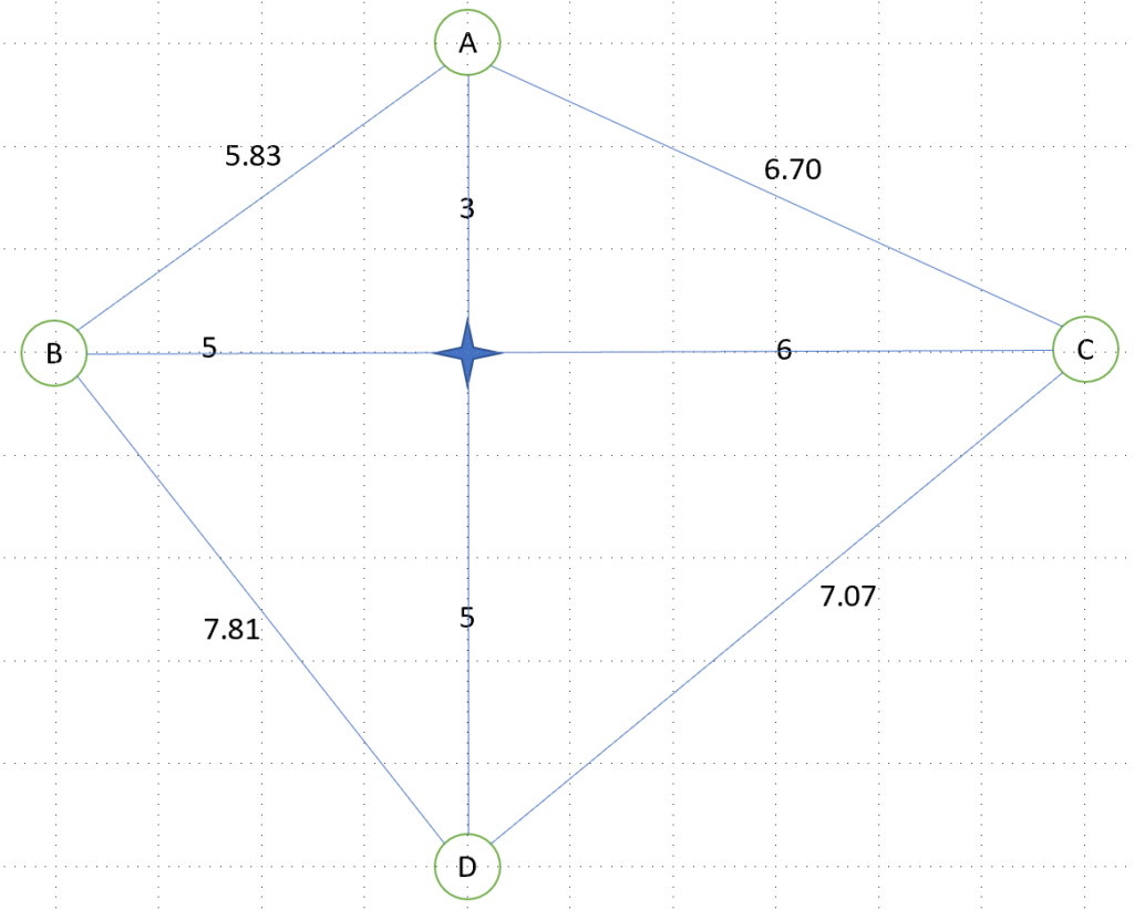
We arbitrarily consider the path city A -> city B -> city C -> city D (implying going back to city A), which has a distance of 5.83+11+7.07+8 = 31.9

The solution is written as a norm, similarly to an RNA sequence, as A-B-C-D

You now have guessed that solution city A -> city B -> city D -> city C (implying going back to city A) would be written as A-B-D-C.

Each following genetic tool will be applied to this TSP problem.

---

Tools of the genetic algorithm

We need 5 basic tools to build a genetic algorithm:

• Initialization
• Selection
• Mutation
• Crossover
• Iteration

---

Tool 1: Initialization

---

Nature context

According to Darwinism, cats have not been created spontaneously. Their ancestor has evolved into leopards and cats. Its ancestor has evolved into pumas and leopards/cats.

To evolve, you always need some starting point(s) called initialization(s).

---

Our TSP application

In our example, genetic algorithms won’t create spontaneous paths.

We need to provide paths.

Basically, we could start from:

• Arbitrarily paths
• Random paths
• Optimized paths (some non-genetic algorithm may already exist and find paths usually better than arbitrarily / random paths)
• …

Application to our TSP example

We arbitrarily choose 3 paths, and write them with « RNA norm sequence format »:

• A-B-C-D
• A-B-D-C
• A-D-C-B

Remark: keep in mind we have chosen to always start from city A.

---

Tool 2: Selection

---

Nature context

In the hereunder diagram, a green tomato and an orange tomato have been selected in order to study the result of their hybridization after one generation (F1), two generations (F2), and three generations (F3)…

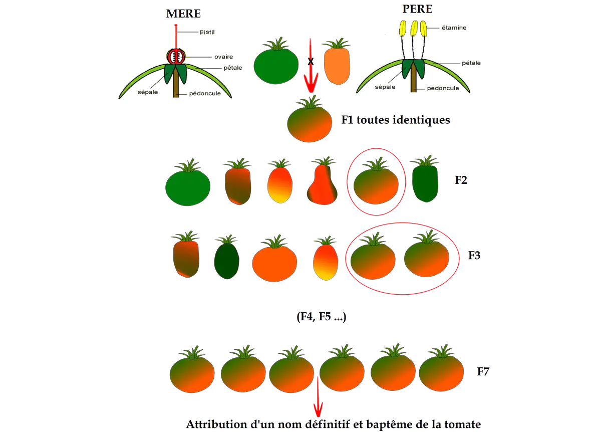
These two initial tomatoes have been selected because they seem promising: « Selection » doesn’t follow any absolute rule.

---

Our TSP Application

We have already defined 3 initialization paths.

We only want to use some of them. With only four cities, we could calculate all solutions. But with many cities, say 1000, it would mean too many calculations, requiring many thousands of years.

The genetic algorithm should be considered when greedy algorithms (algorithms trying to calculate too many solutions) would take too much time. An implied default of genetic algorithm: it could miss the global solution…by not calculating all possible solutions.

The process of selecting some paths from a greater quantity of paths is the selection.

With the genetic algorithm, the selection methods are:

• Choose some of the best paths. Like in nature, it is hoped that the results of good solutions will provide a good solution, and maybe a better solution. These best paths are often called « elite » in program packages
• It is also advised to choose some average solutions, even some bad solutions. The explanation: if you always combine paths with good performance, it may be because these paths are quite similar. There is a risk of being stuck inside a local solution. Indeed, it’s advised to check many different path configurations to hope to find the global solution.

---

Application to our TSP example

As a preparation, we calculate the distance of our 3 initialization paths:

• A-B-C-D: distance of 5.83+11+7.07+8 = 31.9
• A-B-D-C: distance of 5.83+7.81+7.07+6.70 = 27.41
• A-D-C-B: distance of 8+7.07+11+5.83 = 31.9

Now, we arbitrarily choose 2 selection paths, one good and one average. Hence we keep:

• A-B-C-D: Distance of 31.9
• A-B-D-C: Distance of 27.41

Nevertheless, note that this choice may lead to a local solution where B is always the second visited city. And there might be a global solution where C or D is the second city.

A second remark, as the first city (A) is enforced, it means that only 3 cities can be shifted in the paths in the TSP. This lack of openness can quickly lead to a local solution. That’s a side impact of choosing a simple example (only 4 cities) for better understanding.

---

Tool 3: Crossover

---

Nature context

We are focusing on Meiosis.

Meiosis is a process in which a single cell divides twice to produce four cells containing half the original amount of genetic information. These four cells are integrated into eggs in females or into Spermatozoons in males.

What needs to be reminded from the above diagram?

At the start, there is one cell with a navy blue and a light blue chromosome. The two chromosomes are precisely duplicated. Then, they are mixed up: the light blue and the navy blue chromosomes exchange parts of their sequences. In the end, a mainly navy blue chromosome with two parts of light blue is created, and a primarily navy blue chromosome with two parts of navy blue is also created.

In a point of view of data sequence, two sequences are mixed up and recombined as hereunder, let’s detail:

There is a red sequence chromosome (called M), and a blue sequence chromosome (called F). They are crossovered, and this creates two children, C1 and C2.

From a point of view of nature, this crossover may be without impact, or create some evolution, either « good result » or « bad result ».

According to Darwinism, a « good result » has a better chance of survival and of transmitting the new genes to descendants.

---

Our TSP application

Example with ten cities

From A to J: starting from 2 paths, we will try to crossover them

Path 1: A-B-C-D-E-F-G-H-I-J

Path 2: D-B-I-E-A-H-C-J-G-F

–

Basic result and constraint in crossover of TSP

Let’s try to crossover the 3 first cities of 2 parents like in the previous diagram:

A-B-C-D-E-F-G-H-I-J (Parent 1) and D-B-I-E-A-H-C-J-G-F (Parent 2) are mixed according to the bold font: the 2 children would appear as

D-B-I-D-E-F-G-H-I-J (child 1) + A-B-C-E-A-H-C-J-G-F (child 2)

There is an issue: remind that each city must be visited once and only once. As child one is not visiting city A, and child two is not visiting city D, these results are non-sense according to TSP rules.

–

Special TSP ordered crossover

Due to the « each city once and only once » constraint, we arbitrarily define a new TSP crossover rule: first, a sequence from the parent 1 will be arbitrarily chosen (with bold font). Then the remaining sequence will be filled with values from parent 2, in the same order as parent 2, and with removing the duplicates

Example:

A crossover with A-B-C-D-E-F-G-H-I-J (Parent 1) and D-B-I-E-A-H-C-J-G-F (Parent 2) is created, taking into account the fourth/fifth/sixth cities of parent 1

Step 0: the child has the same length as parents, hence its format is:

?-?-?-?-?-?-?-?-?-?

Step 1: the child is filled with the 3 designated cities from Parent 1. Its format is:

?-?-?-D-E-F-G-?-?-?

Step 2:

For this step and all followings, Child must be completed with Parent 2, with respect to the order and to the rule of « no duplicate ».

The first city of Parent 2, D-B-I-E-A-H-C-J-G-F, is D, and already in ?-?-?-D-E-F-G–?-?-?. Hence, city D is skipped, and the building sequence is unchanged.

Step 3:

The second city of Parent 2, D-B-I-E-A-H-C-J-G-F, is B, and is not already in ?-?-?–D-E-F-G–?-?-?. Hence city B is filled at first digit of Child:

B-?-?–D-E-F-G–?-?-?

Step 4:

The third city of Parent 2, D-B-I-E-A-H-C-J-G-F, is I, and is not already in B-?-?-D-E-F-G-?-?-?. Hence city I is filled at second digit of Child:

B-I-?–D-E-F-G–?-?-?

Step 5:

The fourth city of Parent 2, D-B-I-E-A-H-C-J-G-F, is E and is already in B-?-?-D-E-F-G-?-?-?. Hence, city E is skipped, and the sequence is unchanged:

B-I-?–D-E-F-G–?-?-?

…

Final step:

Several steps after, the Child is totally build:

B-I-A–D-E-F-G–H-C-J

–

Variants of crossovers

Others crossovers methods could be applied:

• with random lengths
• on one or more parts
• …

---

Application to our TSP example

We had chosen in the previous part 2 selection paths:

A-B-C-D: distance of 31.9

A-B-D-C: distance of 27.41

Bad luck, it is not possible to combine them. As the sequence is very short, only 4-cities long, it happens! Again a side effect of working with a simple example.

Instead, we change to these 2 paths:

A-B-D-C: distance of 27.41

A-D-C-B: distance of 31.9

One first crossover, A-B-D-C + A-D-C-B:

The initial result is A-B-?-?, and after completing it with the second parent, the final result is A-B-D-C. Its distance is 20 (indeed, we already know this path, chosen in initialization)

One second crossover, A-B-D-C + A-D-C-B:

The initial result is A-D-?-?, and after completing with the second parent, the final result is A-D-B-C. Its distance is 33.51

It is very common to have crossover children not better than the parents, or even worst: we’ll see in tool 5 how to deal with it.

As this 4-cities example is very basic, it is not possible to crossover anymore, and we have to stop at the first iteration. You can generate many iterations of your own with the 10-cities example described in the previous post.

---

Conclusion of Crossover tool

The crossover is a random method, globally similar to nature. For TSP, it allows us to explore many random results/paths.

There is no way to determine if a crossover result/path is promising.

Indeed, with genetic algorithm, when they are too many possibilities, there is a high risk of staying inside local solution.

This random effect must be combined to many trials: hence it allows us to randomly try to check solutions theoretically all around the spectrum.

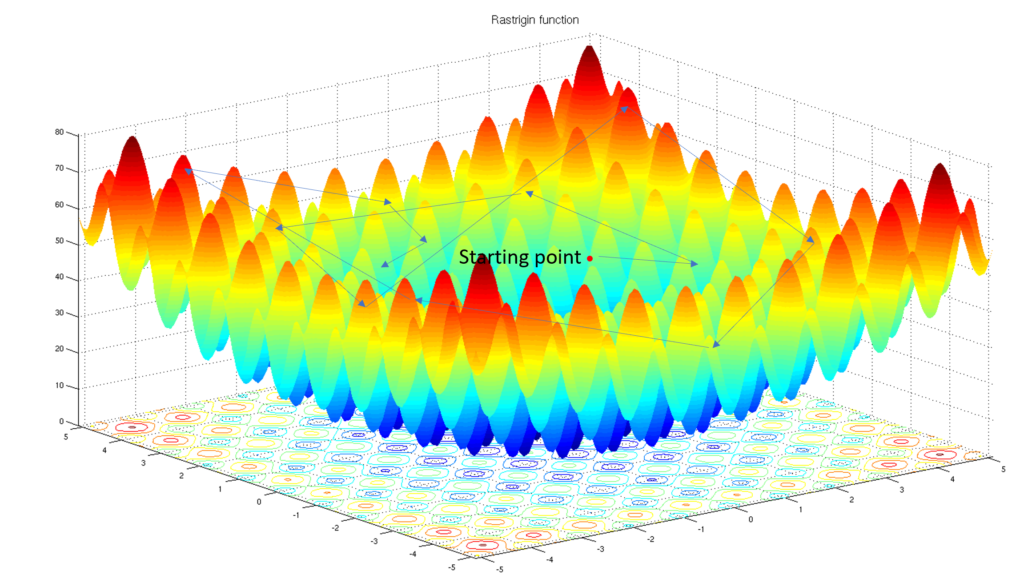
A schematical example: we want to find the maximum value of this Rastrigin function, which is +/- 80.

With a classical algorithm, if you start at an arbitrary point of the map, you might focus on a local solution, +/- 50:

Also schematically, the crossover of the genetic algorithm will test values in a diffuse mode, thanks to its random effect, and it should investigate more local solutions: in this example, a +/- 65 value has been found (trial at top left)

---

Tool 4: Mutation

Nature context

Many types of mutation are possible with Chromosomes:

• Inside the same chromosome, or between two chromosomes
• Deletion, duplication, inversion, translocation of sequences

Indeed, the mutations may occur only at a point, it is called “point mutation”: in the hereunder example, in a sequence of 3 nucleotides, one has been modified due to a mutation.

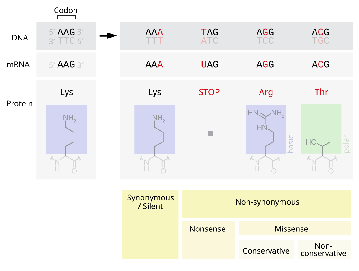
Let’s focus on RNA sequences:

The AAG sequence is the original one: it codes a Lysine protein.

The AAA sequence is silent: despite the modification of the third nucleotide, the original Lysine protein is coded

The UAG sequence, with modification of the first nucleotide, is non-sense for the organism, which is unable to interpret the code.

The AGG sequence is a missense meaning the coded protein has changed to Arginine by the organism. It’s conservative, meaning the Arginine has the same properties as Lysine, the original protein.

The ACG sequence is also a missense: the second protein has changed to Arginine. It’s non-conservative, meaning the Arginine has different properties as Lysine, the original protein.

---

Our TSP application

We have still the constraint that each city must be once and only once in the sequence. Hence, only swaps in paths are allowed.

Some examples with a 10-cities path:

The original path is: A-B-C-D-E-F-G-H-I-J

A mutation could be a minimal swap:

A-B-C-D-E-F-G-H-I-J becomes A-B-C-E-D-F-G-H-I-J

Or a swap/inversion of a longer sequence:

A-B-C-D-E-F-G-H-I-J becomes A-B-C-F-E-D-G-H-I-J

Or a swap between two sequences:

A-B-C-D-E-F-G-H-I-J becomes A-I-J-D-E-F-G-H-B-C

---

TSP example

Arbitrarily, let’s deal with the best path of our initialization:

A-B-D-C: distance of 5.83+7.81+7.07+6.70 = 27.41

We are applying for example 2 mutations:

A-B-D-C becomes A-D-B-C: this new path is already known and has a distance of 33.51

A-B-D-C becomes A-B-C-D: this new path is already known and has a distance of 31.9

It’s a side effect of having a limited number of cities. With a bigger number of cities, interesting solutions might be found!

---

Tool 5: iterations

---

Nature context

Look at the hereunder picture:

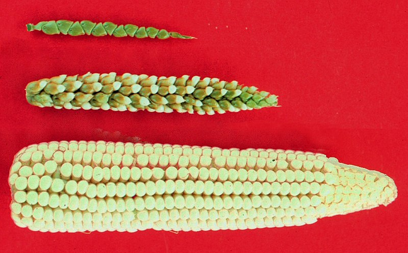
You recognize at third position, the ear of a current maize (corn). Indeed its ancestor is the teosinte, you can note it at the first position; note the very small size of ear of teosinte and its so-small food quantity.

Current “non-Genetically Modified Organism” maize was created by humans, by selecting each year the biggest “ears” of teosinte. Indeed, the biggest ones were the result of mutation. Mutation after mutation the ear of teosinte became bigger and bigger.

9000 years ago, humans were eating ears of teosinte of 2-3 cm

7000 years ago, humans were eating ears of teosinte of 7 cm

2000 years ago humans were eating ears of teosinte (we can call it maize now) of 10 cm

Source: https://mots-agronomie.inra.fr/index.php/Le_ma%C3%AFs,_de_la_t%C3%A9osinte_aux_vari%C3%A9t%C3%A9s_hybrides

Maize is producing ears yearly, and has not been selected every year. Nevertheless, as several thousand years of selection were required, it means that several thousand steps mutations have been needed.

These selection steps are called iterations.

---

Our TSP application

The previous example’s aim with corn genes was to optimize the size of ears of maize: the heaviest ear the better.

Let’s summarize the previous steps:

• With TSP, we need to optimize the path: the smaller distance the better. As we need to initialize any problem resolution: this initialization step can be considered as a pre-iteration.
• Then, at each iteration, a selection is required and then crossovers and mutations are applied.
• We found the best solution in the first iteration because the example is simple and only has four cities.

With a larger number of cities, you can’t except to find the best path at the first iteration. Indeed, later in this post, we’ll check that a genetic program for a 25-city example required 300-400 iterations before finding its best solution.

---

It induces one question with our TSP example: when must we stop the iterations?

With a large number of cities, you cannot calculate all the paths. Hence, you don’t know if you have find the shortest path.

With genetic algorithm, the aim is to find shorter and shorter paths, iteration after iteration.

Some empiric methods in order to stop at the right number of iterations:

• You iterate as much as possible, and stop due to external context: you have no more time allowed, you reach the budget of calculation center…
• You stop iterating when the distance is suitable enough for the business: unhappily this scenario won’t happen often
• You stop iterating, when after a certain number of iterations, no progress is reached at all, or the progress is too small and doesn’t worth to continue

---

Application with Python on our TSP example

In this site https://towardsdatascience.com/evolution-of-a-salesman-a-complete-genetic-algorithm-tutorial-for-python-6fe5d2b3ca35, from Eric Stoltz ( https://towardsdatascience.com/@estoltz ) you will find a python code easy to apply:

• No esoteric package required
• Functions and definitions are well explained if you have at least an intermediary level of Python programming

Copy-Paste in a Python GUI all the blocks with some exceptions.

Don’t copy genetic_algo_14.py. Instead of defining 25 random cities, you will define the 4 cities of our example:

# Here we add respectively the coordinates of cities A, B, C and D
cityList = []
cityList.append(City(x=0, y=3))
cityList.append(City(x=-5, y=0))
cityList.append(City(x=6, y=0))
cityList.append(City(x=0, y=-5))

Don’t copy genetic_algo_17.py. Instead, choose parameters which are adapted to our 4 cities. The initial hyper-paramaters would have raised a greedy calculation.

# At each iteration, we keep 3 paths -> popSize=3
# We keep only two best paths for the next iteration, in order mix with a "deceving" path, in order to avoid a local solution  -> eliteSize=2
# Half of the descendant have mutation -> mutationRate=0.5
# We ask 10 iterations -> generations=10
geneticAlgorithm(population=cityList, popSize=3, eliteSize=2, mutationRate=0.5, generations=10)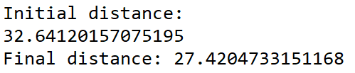

The best path found by the program is 27.42. It is the path A-B-D-C we had found with a distance of 27.41. The small difference is due to the distance, which we round and which is more precise with the program.

Don’t copy genetic_algo_17.py. Use 4-cities proposed parameters, as above:

geneticAlgorithmPlot(population=cityList, popSize=3, eliteSize=2, mutationRate=1, generations=10)

You note that the best solution is found only after one iteration: again the side effect of a simple example with 4-cities.

Then, forcing mutation and cross-over, the following iterations randomly alternate between the optimal solution, and the not-optimized solutions.

This program was not impressive with our 4 cities A, B, C, D.

You should run the program at https://towardsdatascience.com/evolution-of-a-salesman-a-complete-genetic-algorithm-tutorial-for-python-6fe5d2b3ca35 with the default configuration: it is 25 random cities. The genetic algorithm will progress during 300-400 generations and then reach a threshold.

Note that it is not known if the threshold is a limitation of the parameters of the program, or really the best possible solution.

---

Conclusion: do genes inspire Genetic Algorithms?

We have compared and checked that Genetic Algorithms have a natural origin in:

• Initialization
• Selection
• Crossover
• Mutation
• Iterations

Yes, genetic algorithms are inspired by genes.

It should be included in your algorithm toolkit, when problems are too complex to be fully (“greedy”) investigated.

You may expect the genetic algorithm to progress, maybe not quickly, to an optimum, at least progressing to an optimum and providing you a solution, in opposite to some algorithms which would run more or less forevever without providing a solution.