Introduction to dimensionality reduction with Earth map

Let’s consider the earth, it is roughly a sphere :

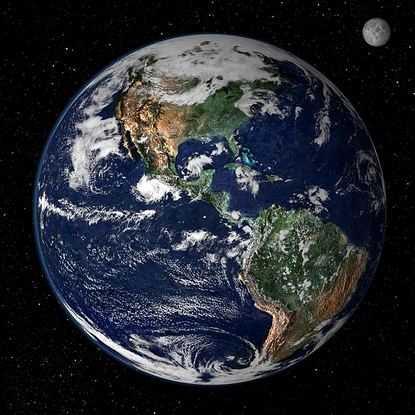
There is a classical challenge :

How to represent the earth, which is modelized with three dimensions?

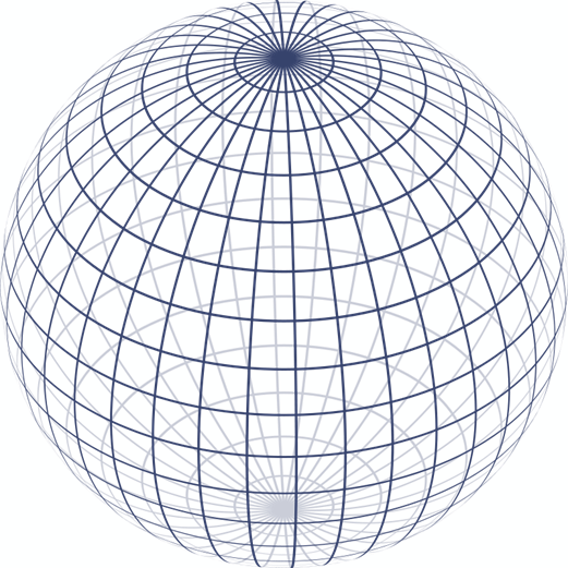
Into a paper or screen map, which is modelized with 2 dimensions?

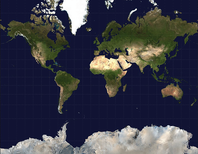
The most common dimensionality reduction map is the Mercator projection

https://en.wikipedia.org/wiki/Mercator_projection

Its main advantages are:

It became the standard map projection for navigation because it uniquely represents north as up and south as down everywhere while preserving local directions and shapes.

https://en.wikipedia.org/wiki/Mercator_projection

Its main default is

As a side effect, the Mercator projection inflates the size of objects away from the equator. This inflation is very small near the equator but accelerates with increasing latitude to become infinite at the poles. So, for example, landmasses such as Greenland and Antarctica appear far larger than they actually are relative to landmasses near the equator, such as Central Africa.

https://en.wikipedia.org/wiki/Mercator_projection

If your main requirement is to compare the areas, you could the Gauss-Krüger projection

https://en.wikipedia.org/wiki/Transverse_Mercator_projection#Ellipsoidal_transverse_Mercator

If you remember the Wikipedia quote about the size of Antarctica / Greenland / Africa: now we really visualize that Africa is bigger than Antarctica, and really bigger than Greenland

---

A quick introduction of dimensionality reduction in data science

The aim of dimensionality is to find a way of visualizing data with many dimensions (for example parameters of observations), it could be dozens, hundreds of dimensions, into:

• mainly 2 dimensions
• rarely 3 dimensions, as it is difficult for human eye to apprehend

Unlike the Earth projection, as there are too many initial dimensions, you usually cannot customize the orientation of the visualization

---

Principles of the t-SNE algorithm

Disclaimer

This algorithm is very complex.

The hereunder explanation is oversimplified, incomplete, and inaccurate, as the aim is to vulgarize:

The target of t-SNE is to transcribe from the source the short distances into the target. In other words, each couple of points close in the high-dimensional will stay close in the low-dimensional

The target of the t-SNE: concept

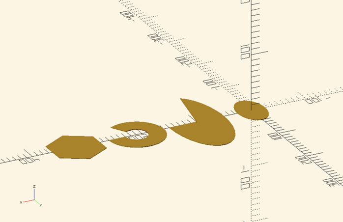
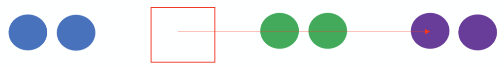
The target of the t-SNE: example

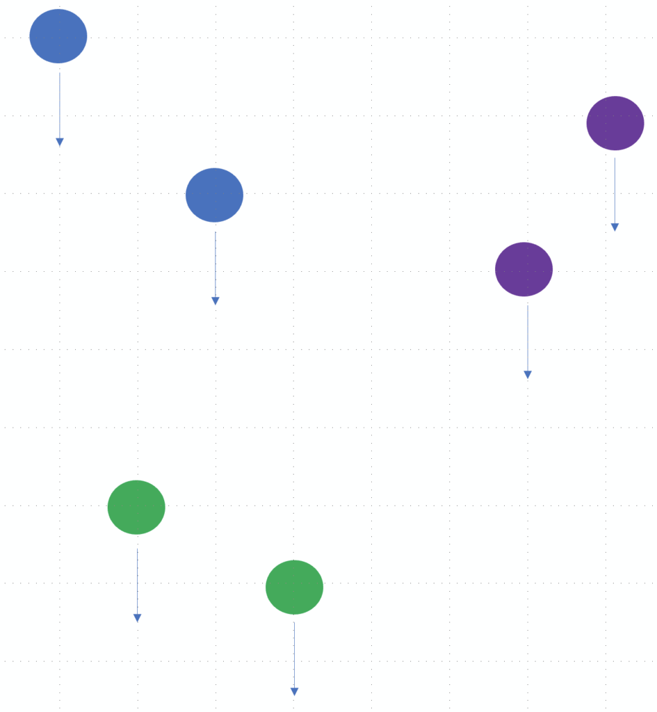
We will try to explain how the hereunder 2-dimension set with 6 observations could be reduced to 1-dimension:

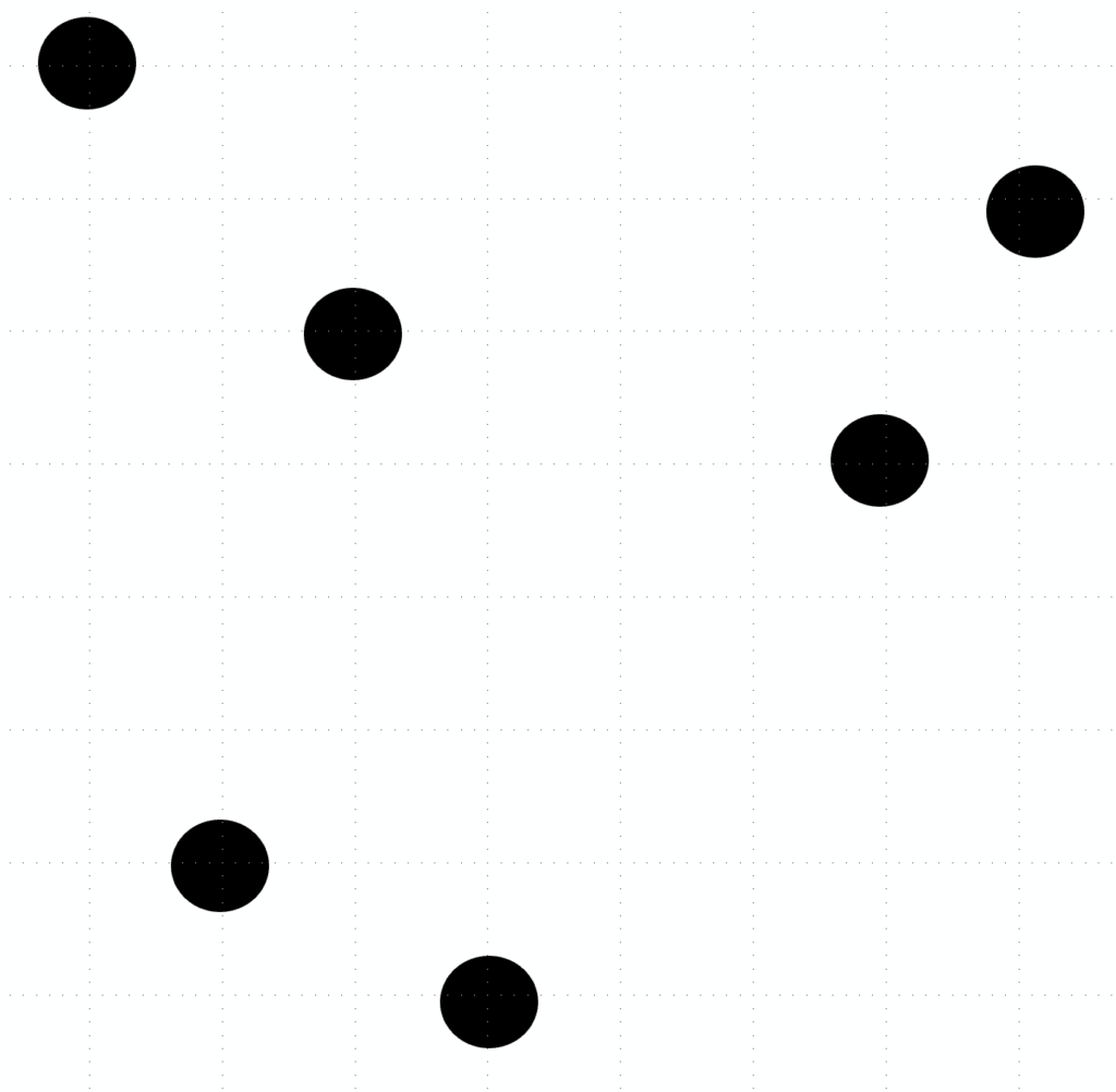
We can notice that we have 3 clusters, indeed there are 3 groups of « close points », each of one containing 2 points.

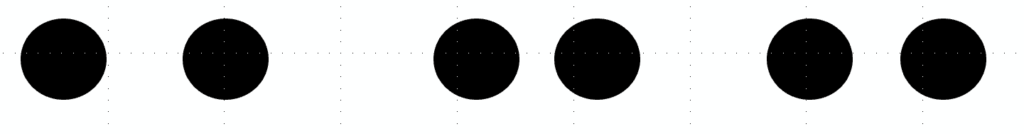
Hence, in the 1-dimension result, we should have 3 clusters of 2 points.

A graphical and empirical result could be as hereunder:

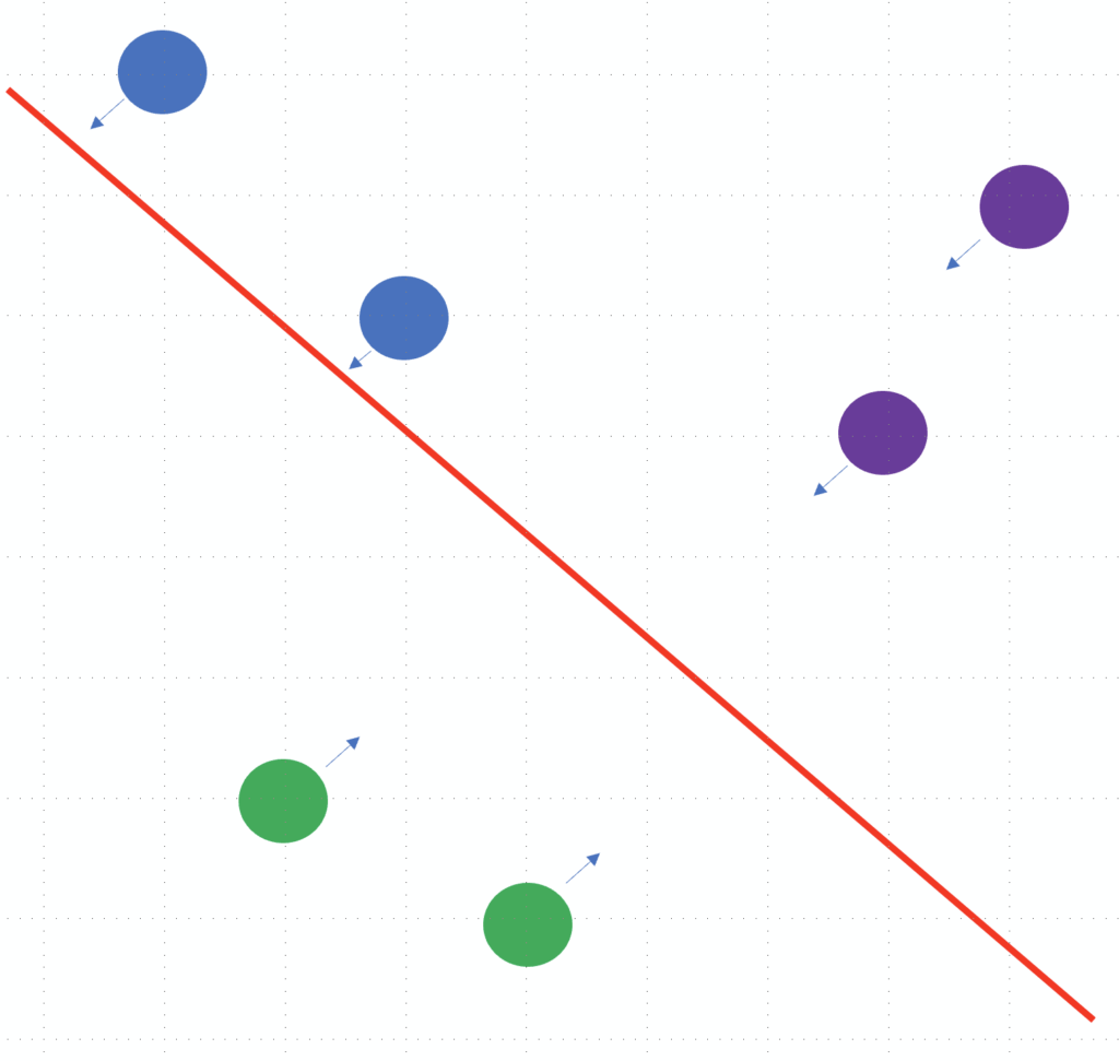
The remark about the non-linearity of t-SNE:

Let’s reshape the initial set with color highlighting the cluster:

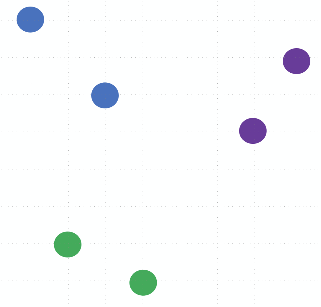
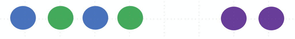
Trial 1: let’s project to an abscissa axis:

The result is

Trial 2: let’s project to an ordinate axis:

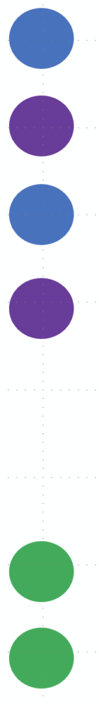
Indeed, any linear projection would bring a good result:

The t-SNE is not linear.

The trick for focusing on small distances: normal distribution and t-distribution

We have explained that each couple of points with a small distance in the source, should have also a small distance in the destination.

It means that we will take into account all the distances of a couple of points, and need to weigh them.

There is an issue: if you work with mathematics with small distances, which are small numbers, and with long distances, which are big numbers, then the long distances naturally have big weights.

The idea is to transform the small distances into big numbers, and the big distances as small numbers, in order to weigh the small distances.

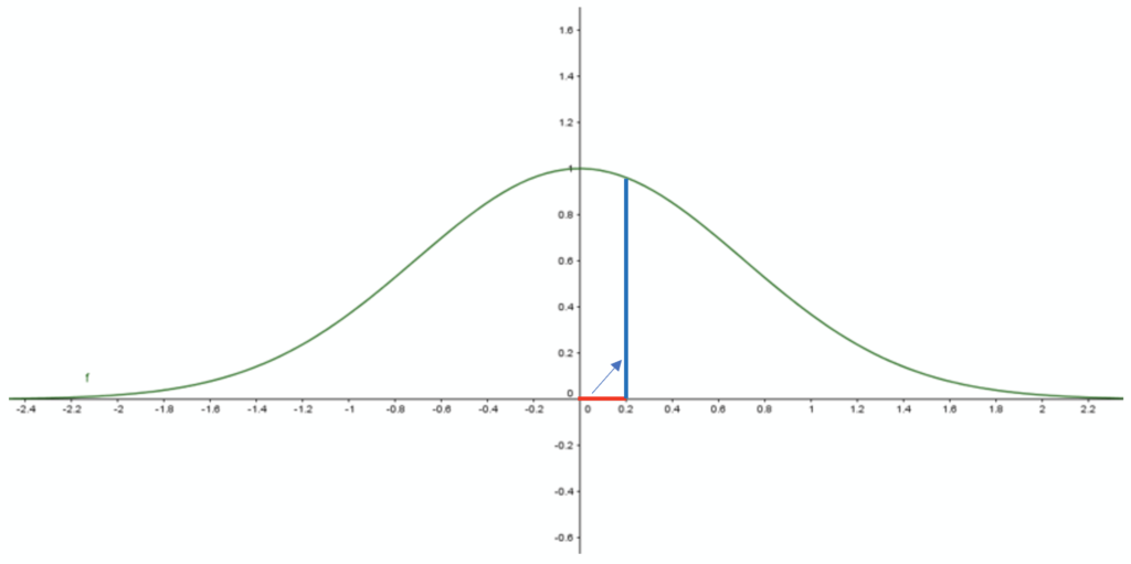
Remind the normal distribution?

Remark: all the hereunder values are totally arbitrary, and are provided in order to simplify the explanation

Let’s imagine we have a short distance of 0.2 in the source set: converted as probability, it would be converted into the target high probability of 0.96:

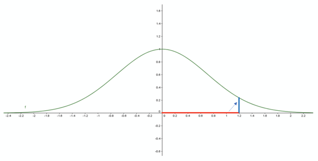
Now, let’s imagine we have a long-distance of 1.2 in the source set: converting as probability, it would be converted into the target small probability of 0.24:

About the destination set, probabilities are converted into distances. This time not with a normal distribution, but with a t-distribution, which has two main differences with normal distribution:

• the top of the t is lower
• the tails of the t are higher

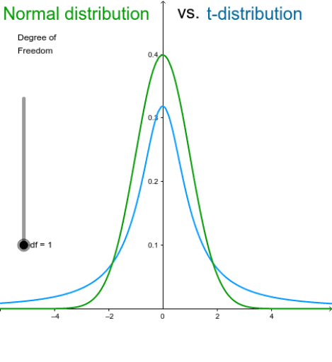
Some details about the t-distribution: https://en.wikipedia.org/wiki/Student%27s_t-distribution

Why a t-distribution instead of a normal distribution? It has been noticed the close points are a good compromise between showing close points but without being too close and hence being visible.

The iterations of t-SNE

The t-SNE doesn’t provide an analytic solution. It uses iteration.

For example, about our example:

At the initial step, the result could be disappointing:

Then the t-SNE focuses on the first point:

• this blue reference point 1 should be closer with the other blue point: highest priority
• this blue reference point 1 should be closer with the two violet point: low priority

Hence, reference point 1 could be moved there:

Then the next iteration focuses on reference point 2:

• this green reference point 1 should be closer with the other gren point: highest priority
• this green reference point 1 has almost similar distance with blue and violet cluster

Hence, reference point 1 could be moved there:

In the new iteration, the violet point would be moved close to the other violet point:

Again, all this t-SNE explanation has been simplified to the max: the target was to popularize this algorithm.

Remark:

Between the first step, where we have focused on the first point, and the sixth step, where we have focused on the sixth point, all points have moved. Hence the position of the first point should be calculated again.

Generally, many many iterations are required, as theoretically, the points are approaching more and more to the t-SNE target: each couple of points close in the high-dimensional will stay close in the low-dimensional

And theoretically again, as the points are approaching more and more to the final position, the shifts are converging.

---

An example of t-SNE visualization with board games

Context

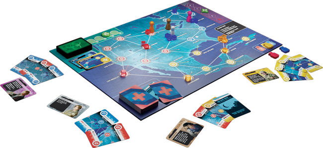
We are considering 22 board games, like Pandemic Hot Zone North America

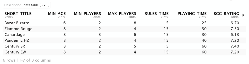
We arbitrarily decide to describe each game with 7 variables/dimensions:

Variable ID	Variable description
MIN_AGE	Minimum age of players [1]
MIN_PLAYERS	Minimum number of players [1]
MAX_PLAYERS	Maximum number of players [1]
RULES_TIME	Rules explanation duration [2]
PLAYING_TIME	Duration of a game [2]
BGG_RATING	Rating from https://boardgamegeek.com/
BGG_WEIGHT	Complexity from https://boardgamegeek.com/

Remark: some variables are correlated. For example, the minimum age and the weight (complexity) of the games

R language solving

First, we load the packages

```{r}
# Load Rtsne package
library(Rtsne)
# Load data.table
library(data.table)
# The ggrepel will solve overlapping issues in text
library(ggrepel)
# ggrepel is used with a ggplot2
library(ggplot2)
```

The dataset of board games can be downloaded there:

The file can be downloaded in R language:

```{r}
# Load the set of observations, which are board games with their properties
dt_games <- fread("C:\\Users\\vince\\OneDrive - Data ScienceTech Institute\\Datascience.lc\\t-sne\\Board games.csv")
# Remove the first column, we keep only the short titles
dt_games <- dt_games[,-1]
head(dt_games)
```

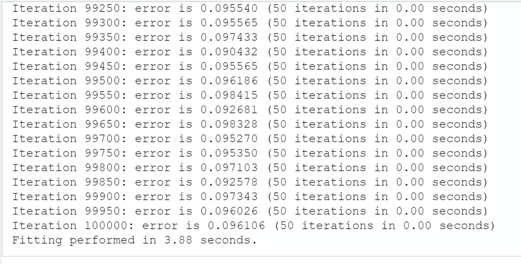
We run the t-SNE algorithm:

```{r}
# We call the Rtsne with following options
# Removing the first column which contains titles 
# We want to display in 2 dimensions
# The perplexity is an hyperparameters which could be close to the number of variables, but not exceeding it
# We are ok to display some log
# A maximum of 1000 iterations
set.seed(2)
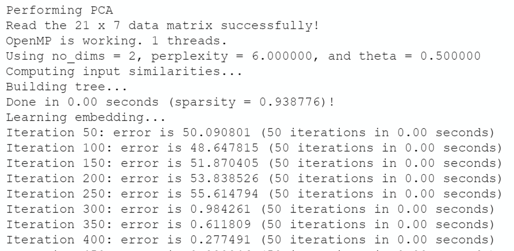
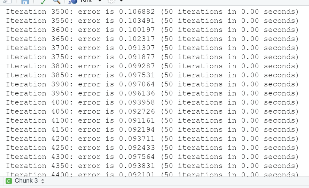
tsne <- Rtsne(dt_games[,-1], dims = 2, perplexity=6, verbose=TRUE, max_iter = 100000)
```

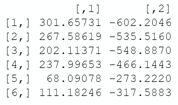
```{r}
# We isolate the coordinates provided by the t-SNE
tsne_coordinates <- tsne$Y
head(tsne_coordinates)
```

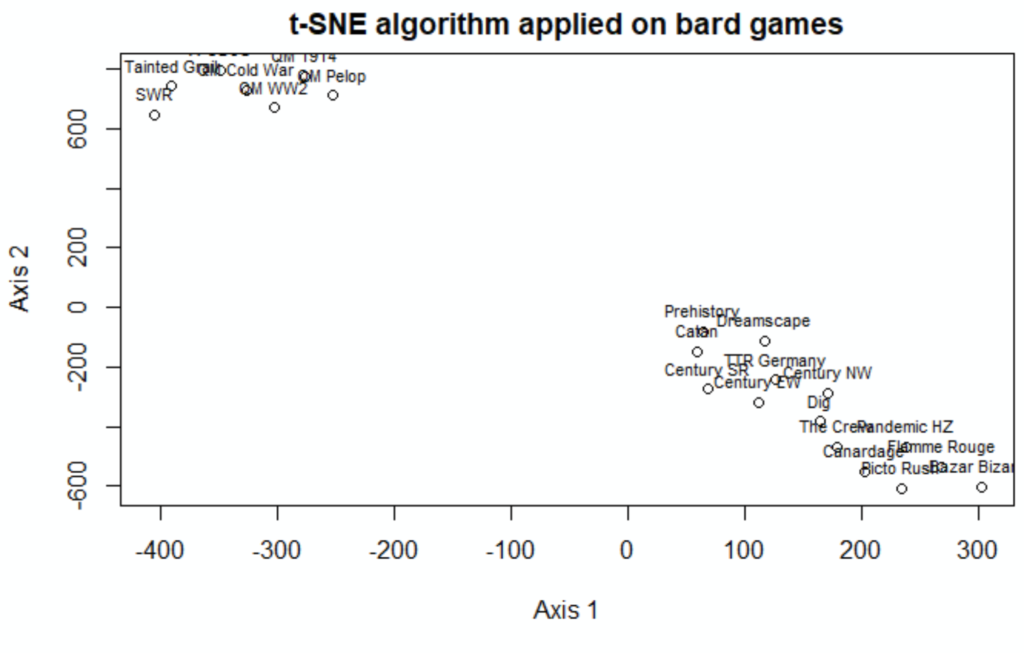
We are ready to plot with 2-dimension:

```{r}
plot(tsne_coordinates, main = "t-SNE algorithm applied on bard games", xlab = "Axis 1", ylab = "Axis 2")
text(tsne_coordinates, dt_games$SHORT_TITLE, cex= 0.7, pos=3)
```

The look and feel can be improved with points in red color and better point title positions.

```{r}
df_tsne_coordinates <- as.data.frame(tsne_coordinates)
ggplot(df_tsne_coordinates, aes(V1, V2, label = dt_games$SHORT_TITLE) ) + geom_point(color = "red") + labs(title = "t-SNE algorithm applied on bard games") + xlab("Axis 1") + ylab("Axis 2") + geom_text_repel()
```

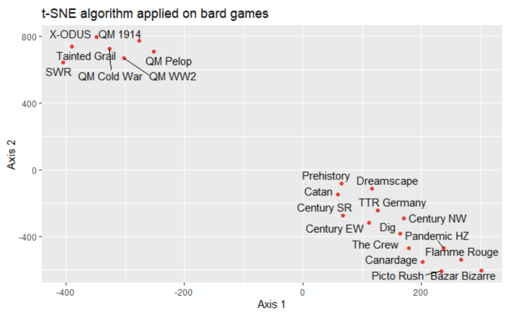
What can be noticed from the 2-dimension visualization?

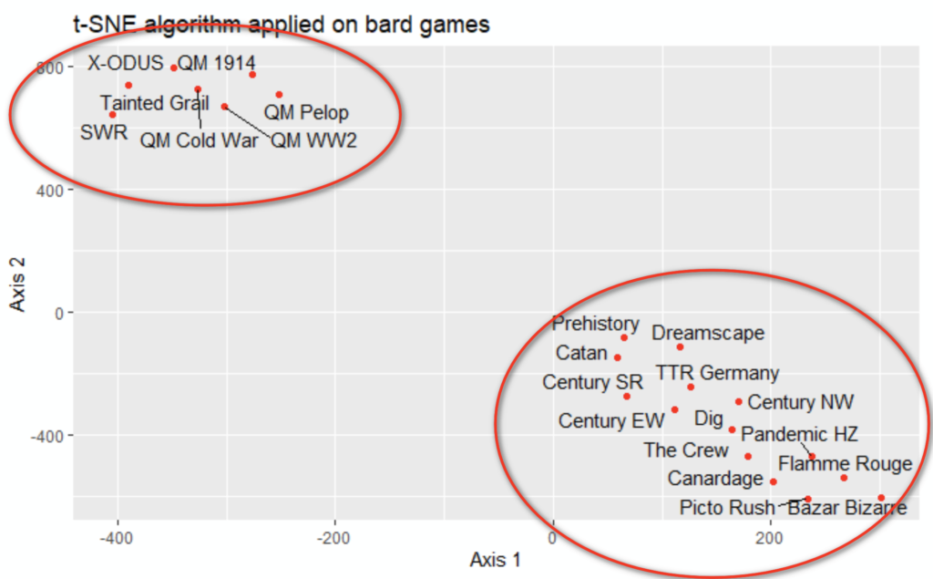
Two clusters are noticed:

• top left, the cluster 1: it looks like the complex games
• above right: it looks like the easy games

It’s consistent with the properties, with two surprises: Dreamscape and Prehistory are « In Real Life » intermediary games

The playing time (80 minutes) is probably the property that brought them in cluster 2 (playing time from 30 to 80 minutes) instead of cluster 1 (playing time from 120 to 300 minutes) or their own cluster

---

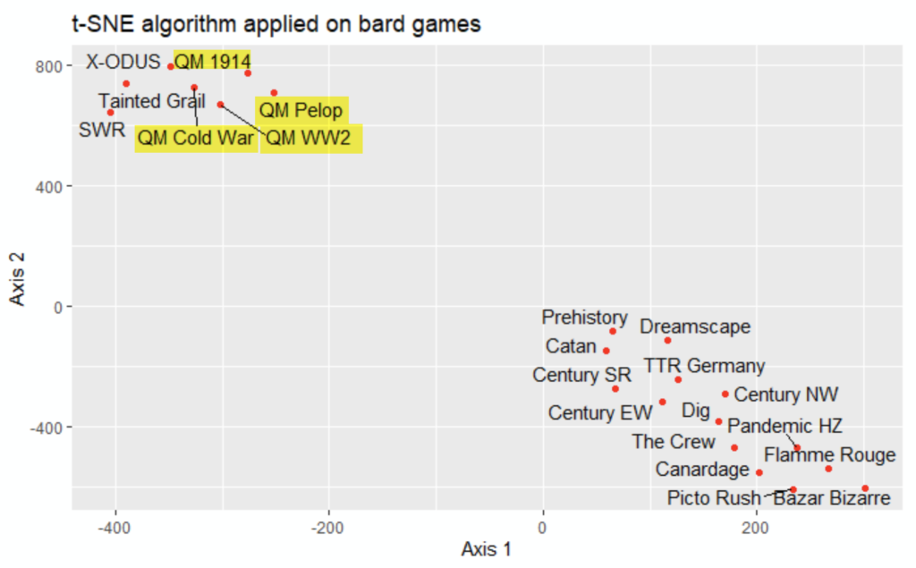
No surprise, the four games of the QM series, have close properties, and hence are close in the 2-dimension visualization

---

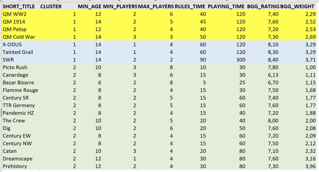
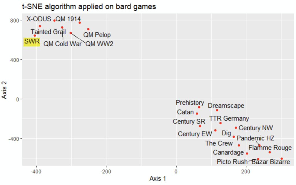
SWR has huge rules times & playing times compared to the other games, and is the only one with 2 maximum players (according to the author o this post): we could have imagined it with its own cluster

Indeed, it has a minimum age, rating, and weight not so far from the other games of cluster 1, which is a fair only explanation.

---

Conclusion

Let’s remember its name comes from:

• t-distributed: this is a probability function involved for calculation
• stochastic: applied to the above function, the distances have been converted into probabilities
• Neighbor: if you add only one word to remember: two points close in high/source dimension are also close in low/target dimension
• embedded: reminds the dimensional reduction with a mathematics word: A map which maps a subspace (smaller structure) to the whole space (larger structure) https://en.wiktionary.org/wiki/embedding

Th t-sne algorithm allows visualizing data originally with many dimensions, usually into a 2-dimension.

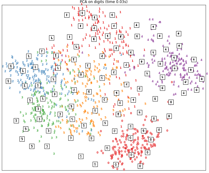
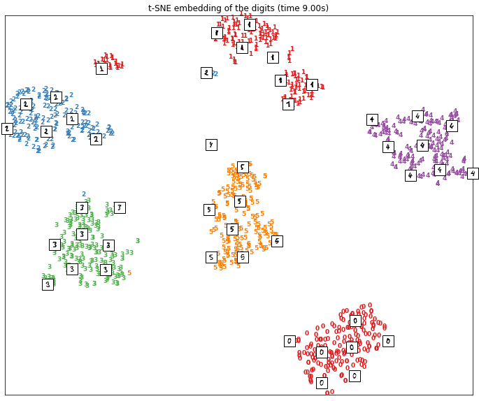
The t-sne algorithm should belong to your dimensionality algorithm toolbox. As proof, let’s display its result, compared to the classical PCA Principal Component Analysis algorithm, about 2-dimension visualization of the famous handwritten digits database MNIST

The t-nse algorithm is remarkably clustering the digits, from 1 to 9:

Its usual competitor, the PCA algorithm, https://en.wikipedia.org/wiki/Principal_component_analysis, is definitely less efficient with the MNIST database: