---

---

Concept of Simplex Algorithm

---

Definition

The simplex algorithm is an algorithm solving linear optimization problems

---

What is a linear equation?

Examples of linear functions:

$f(x) = 1$

$f(x) = -3x$

$f(x) = 2x +4$

$f(x,y) = 2x -4y +4$

Examples of linear equations:

$f(x,y) \leq 0$

$f(x,y) > 0$

$f(x,y) = 0$

---

Examples of NOT-linear functions:

$f(x) = 3x^2$

$f(x) = 3.ln(x)$

$f(x) = 1/x$

---

What is a linear problem?

It consists of 3 parts:

• A linear function to be maximized or minimized – mandatory (*)
• Problem constraints – optional (**)
• Non-negative variables – optional (***)

---

Example of aconversion of a simplified use case into a linear problem

The example is filling a truck with pallets of Product A and Product B

The requirement is:

• Maximize the truck shipment value
• Each pallet of product A is sold 200€, each pallet of product B is sold 300€
• The truck contains up to 10 pallets
• In stock, there are only 5 pallets of product A, and 8 pallets of product B

The maths translation is:

The 2 variables x and y are respectively the number of pallets A and B

(*) Maximize $f(x,y) = 200x + 300y$

(**) $x \leq 5$

( **) $y \leq 8$

(**) $x + y \leq 10$

(***) $x \geq 0$ It is implied for a human, not for the simplex which could find a negative value

(***) $y \geq 0$ It is implied for a human, not for the simplex which could find a negative value

Remark: Simplex deals with continuous variables and provides solutions x and y as real numbers. If it is not allowed to divide the content of a pallet, the real numbers need to be manually converted into integer numbers that are relevant to all constraints.

---

Graphical example of a linear problem with 2 variables

---

We want solve this problem:

• Minimizing the function$f(x,y) = 4x + 5y + 1$
• With 4 constraints
  • $-2x -y -1 \leq 0$ (1)
  • $2x -y -1 \leq 0$ (2)
  • $-1/2x -y + 3/2 \geq 0$ (3)
  • $1/2x -y + 1 = 0$ (4)

---

Rearrangement of the constraints equations

Hence, it will be easier to draw these equations

• $-2x -1 \leq y$ (1)
• $2x -1 \leq -y$ (2)
• $-1/2x + 3/2 \geq y$ (3)
• $1/2x + 1 = y$ (4)

---

Procedure

On a graphic, we draw the constraint « limits », which are lines. Then we mark as removed the areas outside the constraints with grey color. Hence, the constraint-compatible areas will be kept in white color.

In case of multiple constraints, only the white parts are kept.

If the constraint is a equality: the solution is the line itself
If the constraint is an inequality: the solution is an area, excluding the line in case of strict operator . With the constraints like $\geq$ or $\leq$, the lines themselves are kept. With $\ge$ or $\le$ , the lines are excluded

---

Step 1: constraint 1

We draw $f(x) = -2x -1$  and we remove the lower part defined by the line as the right area is $f(x) \geq y$ with grey color:

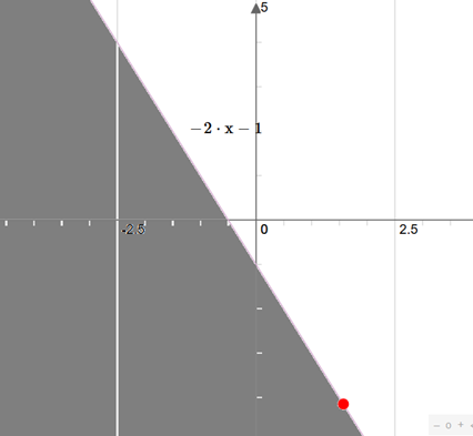
Tip: if you doubt choosing the upper/lower area corresponding to the inside/outside constraint, pick an arbitrary point like (x=1,y=5)  => as -2*1-5-1=-8 and as -8 < 5; this point is inside the constraint. As this inside-constraint point is graphically on top of the line, the upper area on top of the line is ok.

---

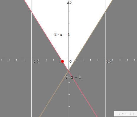
Step 2: constraint 2

We draw $f(x) = 2x -1$  and we remove the lower part defined by the line as the right area is f(x) >= y with grey color:

---

Step 3: constraint 3

We draw $f(x) = -1/2x + 3/2$ and we remove the upper part defined by the line as the right area is f(x) <= y with grey color:

---

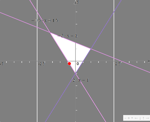
Step 4: constraint 4

We draw $f(x) = 1/2x + 1$, and we keep in red the part defined in the white area, as the new proper constraint is $f(x) = y$ :

Hence, the solution belongs to this red segment between these 2 points:

• Point 1 (x, y) = (0.50, 1.25)
• Point 2 (x, y) = (-0.8, 0.6)

---

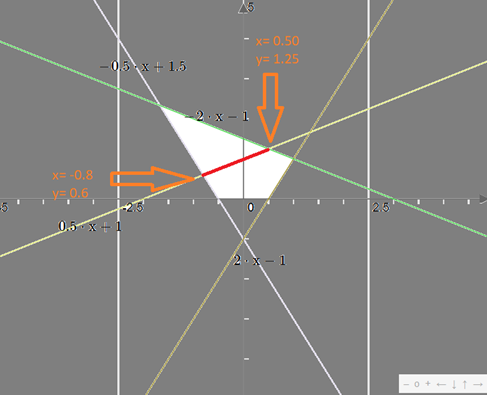
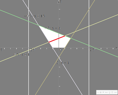
Step 5: finding the minimum of the function

The function we want to minimize is $f(x,y) = 4x + 5y + 1$ is a linear function.  As a consequence, it’s either increasing, decreasing or constant function when navigating through a segment from a extremity to the other extremity

The solution is at one of the two extremities of the segment, or on all this segment; let’s calculate the extremities values:

f(-0.8,0.6) = 4*-0.8 + 5*0.6 + 1 = 0.8

f(0.5,1.25) = 4*0.5 + 5*1.25 + 1 = 9.25

Hence the minimum of f(x,y) according to the four constraints is with x=-0.8 and y=0.6, and the value of the function is 0.8

---

Summary of the Simplex Algorithm definition

A linear problem is analytically solved by the simplex algorithm.

Analytical means a precise method which provides the optimal solution (in opposite to an optimization which would use iterations, giving a numeric solution and maybe providing a local solution and not the global solution )

The simplex algorithm starts at one vertex and calculates the value of the function to minimize or maximize at this vertex. It finds all vertices adjacent to this vertex, calculates the value of the function we want to minimize or maximize, and finds the best new vertex. It iterates to a new vertex until no better vertex has been found, meaning all constraints have been checked.

We have seen graphically the main steps to solve a linear function with 2 variables.

---

Enhancing the simplex algorithm to more than 2 variables

For any N variables in the function to optimize and the constraints functions, the simplex method like the graphical example, can be schematized with figures :

• the constraints with N variables are drawing a polytope with N dimensions
• the solution is at one vertex, due to the property of linear functions

---

Simplified graphical simplex with 3 dimensions: minimizing a cost function

Context:

• The aim is to follow the concept with one more variable
• Thus, we are working on a very simplified and schematized genuine graphical example
• We don’t know the inequality constraint functions, we only know they already have been graphically applied in the hereunder polytope, and the solution area is inside this polytope. They already have been drawn as below
• We want to minimize a not-known linear cost function. The values of the cost function depending on the [x,y,z] position will be given when needed.

Step 1:

We start at one arbitrary vertex (usually determined by the order of the constraints) with a cost function value = 20

Step 2:

We calculate all adjacent vertex values of the cost function, let’s assume the results are 18 (up vertex), 22(right vertex) and 24 (rear vertex).

The vertex with fewer cost value is 18, hence we navigate to it

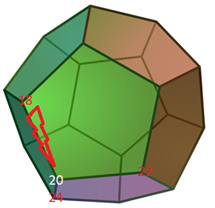
Step 3:

We calculate all adjacent vertice values of the cost function, let’s assume the results are 17 (up/right vertex) and 19 (rear vertex).

The vertex with fewer cost value is 17, hence we navigate to it

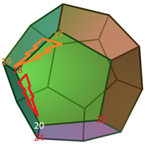
Step 4:

We calculate all adjacent vertex values of the cost function, let’s assume the results are 19 (rear vertex) and 24 (right/down vertex).

No adjacent vertex has a better cost value. We have now the solution, meaning the coordinates of the vertices, and the best function value possible

Summary:

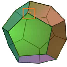
The solution value  of the cost function is 17

The coordinates solution in the form [x,y,z] are according to the point with value 17 defined by the black arrow

---

Graphical simplex with four and more variables

Bad luck, it is not possible to draw in 4 dimensions. It leads to the next paragraph

---

Generalized application of simplex

Whatever the number of variables, the simplex algorithm involves a matrix calculation, using a pivot which is a slide between vertice like in 3D graph: this method is described step-by-step there: https://www.imse.iastate.edu/files/2015/08/Explanation-of-Simplex-Method.docx

---

Programming application of the simplex method

It is not needed and not advised to redevelop the above algorithm, as many tools/libraries for many languages and software are provided.

Indeed they usually don’t have the same power or functionalities: some of them have an optimized algorithm and can deal with a great number of variables, and are quicker.

Free solution

For example, in R, rcbc library is very efficient. It needs a little implementation effort, as it is not part in the CRAN.

Licenced solution

If R/Python/C++/C libraries are not enough, some commercial software are available, like CPLEX.

---

Solving the first 2 variables example with R language

Reminder:

Objective: mMinimizing the function$f(x,y) = 4x + 5y + 1$

With 4 constraints :

• $-2x -y \leq 1$
• $2x -y -1 \leq 0$
• $-1/2x -y + 3/2 \geq 0$
• $1/2x -y + 1 = 0$

```{r}
# calling the libraries
library(Matrix) # used for formatting the input data to the rcbc library
library(rcbc)   # the core library for solving the simplex
```

```{r}
# function to minimize: 
# f(x,y)= 4*x+5*y+1 is equal to minimize f(x,y)= 4*x+5*y
minimize <- c(4,5)
```
# set up of the constraints in a format known by rc: 
# in first column: x coefficient; in second column: y coeficient
# row 1 to 4: the constraints

```{r}
matrice <- matrix( c(-2,-1,2,-1,-0.5,-1,0.5,-1),ncol = 2, nrow = 4, byrow=TR)
print(matrice)
```

We check the matrix constraint content:

     [,1] [,2]
[1,] -2.0   -1    # new format of "-2x -y" 
[2,]  2.0   -1    # new format of  "2x -y"
[3,] -0.5   -1    # new format of "-1/2x -y"
[4,]  0.5   -1    # new format of "1/2x -y"

# the boundaries of the 4 constraints rows: can manage <=, >=, and =
# row_min for the minimum
# row_max for the minimum
```{r}
row_min <- c(-Inf,-Inf,-1.5,-1)
row_max <- c(1,1,Inf,-1)
print(row_min)
print(row_max)
```

We check the rows:

[1] -Inf -Inf -1.5 -1.0
[1]   1   1 Inf  -1 
# Inf means + infinity means there is no upper boundary 
# -Inf means – infinity means there is no lower boundary 
# the First column means "-2x -y" is between -Infinity and 1
# the Second column means "2x -y" is between -Infinity and 1 
# Third column means "-1/2x -y" is between -1.5 and +Infinity
# the Fourth column means "1/2x -y" is between -1 and -1, meaning equal to 1

We prepare the potential future error messages: please note all the reasons why a simplex calculation could fail

```{r}
# Error messages
mip_status <- function(status_code) {
  if (status_code == "optimal") {
    cat("Proven Optimal")
  } else if (status_code == "unbounded") {
    cat("Proven Dual Infeasible")
  } else if (status_code == "infeasible") {
    cat("Proven Infeasible")
  } else if (status_code == "nodelimit") {
    cat("Node Limit Reached")
  } else if (status_code == "solutionlimit") {
    cat("Solution Limit Reached")
  } else if (status_code == "abandoned") {
    cat("Abandoned")
  } else if (status_code == "iterationlimit") {
    cat("Iteration Limit Reached")
  } else if (status_code == "timelimit") {
    cat("Seconds Limit Reached")
  } else if (status_code == "unknown") {
    cat("Unknown")
  } else {
    cat("Status unknown")
  }
}
```

We run the simplex calculation:

```{r}
system.time({
  status_code <- cbc_solve(obj = minimize,
                           mat = matrice,
                           is_integer = rep(FALSE, times = 2),
                           row_lb = row_min,
                           row_ub = row_max,
#                           col_lb = col_min,
#                           col_ub = col_max,
                           max = FALSE,
                           cbc_args = list(sec = 3600,
                                           PassP = 10))
})
```

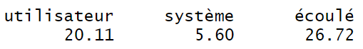
Here we get the summary of the calculation, not yet the solution:

Wutilisateur elcome to the CBC MILP Solver 
Version: 2.9.8 
Build Date: May  8 2017 

command line - problem -sec 3600 -PassP 10 -solve -quit (default strategy 1)
seconds was changed from 1e+100 to 3600
passPresolve was changed from 5 to 10
Presolve 0 (-4) rows, 0 (-2) columns and 0 (-8) elements
Empty problem - 0 rows, 0 columns and 0 elements
Optimal - objective value -0.2
After Postsolve, objective -0.2, infeasibilities - dual 0 (0), primal 0 (0)
Optimal objective -0.2 - 0 iterations time 0.002, Presolve 0    système .00
Total time (CPU seconds):       0.00   (Wallclock seconds):       0.00

     écoulé 
          0           0           0 

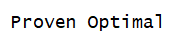
We ask for the status code:

#  Status Code
```{r}
mip_status(solution_status(status_code))
```

The status code indicates everything is fine:

Proven Optimal

We ask the solution:

# Value of function to optimize
```{r}
objective_value(status_code)
```

The solution is the minimal value of $f(x,y) = 4x + 5y + 1$ according to the constraints

[1] -0.2

We ask the values of (x, y) linked to this solution:

# Solution: what are the values of the different variables?
```{r}
column_solution(status_code)
```

The answer:

[1] -0.8  0.6

It means the point [x= -0.8 and y=0.6] is the solution

---

Interest of simplex algorithm

Yes, your company/customer won’t have so many optimization linear problems, many of them are non-linear.

Nevertheless, when they are linear, you get the warranty of analytic solution.  

And with the right free libraries, you can deal with dozen of thousands of variables

---

Hydropower example of Simplex Algorithm

---

Not already convinced by simplex for a company use case?

Aim of the Hydropower example

This article aims to show with an industry scenario how the Simplex algorithm could help your company/client

---

Description of the hydropower plant scenario

The aim is to maximize the yearly revenue of a hydropower plant consisting of 2 turbines p and q producing energy: during one year, hour after hour, the operation of each 2 turbines must be tuned in a range between « no production » to « full production »

Reminder: there are 8760 hours in one standard year

This hydropower plant is supplied by one water reservoir.

The reservoir has a maximum water volume of 25000000 m³. At the beginning of the year, the water volume is 12500000 m³

This reservoir volume is modified by:

• Loss due to leaks: 2 m³/s.
• Gain trough streams as water supplies. The yearly contributions have already been forecast: thanks to previous data and machine learning, we already know the future hourly contribution of the streams next year, hour after hour
• Consumption by the 2 turbines, if turned on during the considered hours

The 2 stream supplies

Small extract of water supply	Supply (m3/s)
Hour 1	24.367
Hour 2	24.367
Hour 3	24.367
Hour 4	24.367
…	…

The turbines

Each 2 turbines p and q is working independently.

• Turbine p is operating in a range from 0 m³/s to 230 m³/s , with tuning each hour
• Turbine q is operating in a range from 0 m³/s to 180 m³/s , with tuning each hour

Turbines p and q are producing energy in MWh (MWh meaning a power of one Megawatt produced during one hour), according to the following rules:

• Energy produced by turbine p in MW.h during one hour is its water flow multiplied by a coefficient of 1.07
• Energy produced by turbine q in MW.h during one hour is its water flow multiplied by a coefficient of 1.01

Turbines p and q sell energy according to a spot price, determined in € / MWh, which changes every hour and has already been forecast thanks to previous data and machine learning; hence, we already know the future hourly spot price of the turbines for the next year.

Small extract of spot price	Prices(Eur/MWh)
Hour 1	19.801
Hour 2	20.481
Hour 3	20.411
Hour 4	14.335
…	…

The data files

This file contains as columns:

• hours from 1 to 8760
• supply in m³/s
• spot price in EUR/MWh

---

Simplex point of view: focus on variables, function to optimize and constraints

The variables to be determined are the hourly flows of each turbine, which will be called flow_p(h) and flow_p(h)

• 8760 variables for the turbine p, for each hour of the year, define the flow of this turbine, inside its min/max operational range. We will call the flow of turbine p depending of the time: flow_t(h), h between 1 and 8760
• 8760 variables for the turbine q, for each hour of the year, define the flow of this turbine, inside its min/max operational range. We will call the flow of turbine q depending of the time: flow_q(h), h between 1 and 8760

This is a total of 17520 variables to solve

Remark: why h between 1 and 8760 , an not h between 0 and 8759? Indeed both are a good solution. [hour = 1) is starting at 0 (hour) and finishes at 1 (hour), so both methods are relevant

In my case, as I use R language to develop the solution, and as in R language, the first row of a data table is 1, it is easier. With Python, it would have been different, as the first row is o.

The function to maximize is the accumulated revenue of 2 turbines producing energy, during one year, we have 17520 variables

$yearlyRevenue(flow_p0001, flow_q0001,..., flow_p8760, flow_q8760) = \sum_{h=1}^{8760} revenue_p(h) + revenue_q(h)$

The volume(h) must be between 0 and 25000000 m³

It depends on:

• as input: water supplies supply(h)
• as output: turbine flows flow_p(h) and flow_q (h)
• as output: leaks

---

Schema

---

Detailing the function to maximize

Intermediary information: the hourly energy production

At one hour h, with h between 1 and 8760, the energy production is:

$energy_p(h) = flow_p(h) * 1.07$

$energy_q(h) = flow_q(h) * 1.01$

Intermediary information: the hourly energy revenue

At one hour h, with h between 1 and 8760, the revenue is: $revenue(h) = revenue_p(h) + revenue_q(h)$

$revenue(h) = flow_p(h) * 1.07 * spotprice(h) + flow_q(h) * 1.01 * spotprice(h)$

Finally the function to optimize

This is the yearly revenue function, and we want to maximize it:

$yearlyRevenue(flow_p0001, flow_q0001,..., flow_p8760, flow_q8760) = \sum_{h=1}^{8760} ( flow_p(h) * 1.07 + flow_q(h) * 1.01 ) * spotprice(h)$

---

Formatting the turbines’ constraints

They are translated as:

• $0 \leq flow_p(h) \leq 230$
• $0 \leq flow_q(h) \leq 180$

Later we will set them up into a format recognized to the rcbc library in R language, we will come back to this shaping :

	Minimum	flow_p(1)	flow_q(1)	flow_p(2)	flow_q(2)	…	…	Maximum
h = 1	0	1						230
h = 1	0		1					180
h = 2	0			1				230
h = 2	0				1			180
…								…
…								…

The reservoir volume raw constraints

The volume has a minimum: it must be positive, it’s obvious for a human, not for a simplex calculation who could find a negative solution

The volume has a maximum: 25000000 m³

The reservoir volume reshaped constraints

The previous constraints must be reshaped:

• We don’t need to know the volume. Precisely, Simplex algorithm doesn’t need this information and doesn’t want this information. The explanation: Simplex algorithm is only able to solve the problem according information linked to the 17520 variables which are flow_p(1), … ,flow_p(8760), flow_q(1), … ,flow_q(8760)
• The constraint must be translated in a math way for each hour h between 1 and 8760

The initial target is now to calculate the volume(h) with h between 1 and 8760

Remarks:

The volume is to be considered at the end of the hour.

We have the initial volume(0) at start of the year, volume(0) = 12500000 m³

And after the first hour is completed, meaning ending h=1, we have a new volume volume(1)

Describing the volume at one hour h depending on the volume at hour h-1

It’s how we are setting into equation the volume by applying the main rule of chemical engineering.

---

Considering the reservoir:

Accumulation = Input – Output

$Volume(h) – Volume(h-1) = Water inputs (h) – Water outputs(h)$

Water inputs: supply from rain

Water outputs: the leaks and turbines’ consumption

$Volume(h) = Volume(h-1) + supply(h) – loss(h) – flow_p(h) – flow_q(h)$

Example of volume constraints for hour h=1

$volume(1) = volume(0) – loss(1) + supply(1) – flow_p(1) – flow_q(1)$

And as $0 \leq volume(1) \leq 25000000$ :

$-25000000 \leq – volume(0) + loss(1) – supply(1) + flow_p(1) + flow_q(1) \leq 0$

Math trick: we have above multiplied with -1, it’s why the minimum term and the maximum term have been shifted

Meaning:

$-25000000 – ( – volume(0) + loss(1) – supply(1) ) \leq flow_p(1) + flow_q(1) \leq 0 – ( – volume(0) + loss(1) – supply(1) )$

Meaning:

$-25000000 + volume(0) – loss(1) + supply(1) ) \leq flow_p(1) + flow_q(1) \leq 0 + volume(0) – loss(1) + supply(1)$

Meaning:

$-25000000 + 12500000 – 2*3600 + 24.367 * 3600 \leq flow_p(1) * 3600 + flow_q(1) * 3600 \leq 0 + 12500000 – 2*3600 + 24.367 * 3600$

We divide each group per 3600:

$-25000000 / 3600 + 12500000 / 3600 – 2+ 24.367 \leq flow_p(1) * + flow_q(1) \leq 0/ 3600 + 12500000 / 3600 – 2+ 24.367$

Final result:

$-3449,855222 \leq flow_p(1) + flow_q(1) \leq 3494,589222$

Lost ? Forgotten why so many math transformations?

As a summary, we have managed to present the constraints only according to flow_p(1) and flow_q(1)

New target: generalization of the volume constraint for all hours h

Hereunder was an example, and only applicable to the first hour. We need an application for each 8760 hours of the year

Just remember that with volume constraint, for each h between 1 and 8760:

• we have a minimum and a maximum boundaries
• at h = 1 it depends on flow_p(1) and flow_q(1)
• at h = 2 it depends on flow_p(1) and flow_q(1) and flow_p(2) and flow_q(2) due to recursive calculation of reservoir volume
• at h = n it depends on flow_p(1) and flow_q(1) and flow_p(2) and flow_q(2) and …. and flow_p(n-1) and flow_q(n-1)
• For simplex programming in R with rcbc library we have to express it as matrix like:

	min value	flow_p(1)	flow_q(1)	flow_p(2)	flow_q(2)	…	max value
for h = 1	?	1	1				?
for h = 2	?	1	1	1	1		?
for h = 3
for h = 4
…
for h = 8760

Job of generalization of the volume constraint for all hours h

The constraint is $0 \leq Volume(h) \leq 25000000$

Meaning:

$0 \leq volumeInitial + ∑ supply * 3600- ∑ loss * 3600 – ∑ flow_p * 3600 –  ∑ flow_q * 3600 \leq 25000000$

Meaning:

$0 / 3600 – volume_initial / 3600 – ∑ supply + ∑ loss \leq – ∑flow_p –  ∑ flow_q  \leq 25000000 / 3600 – volumeInitial / 3600- ∑ supply+ ∑ loss$

Meaning:

$0 / 3600 + volume_initial / 3600 + ∑ supply- ∑ loss >=  + ∑ flow_p +  ∑ flow_q  \leq – 25000000 / 3600  + volumeInitial / 3600 + ∑ supply- ∑ loss$

Meaning:

$– 25000000 / 3600  + volume_initial / 3600 + ∑ supply – ∑ loss \leq + ∑flow_p +  ∑flow_q   \leq 0 / 3600 + volumeInitial / 3600 + ∑ supply – ∑ loss$

Trick: in R program, the function of cumulated sum cumsum will be used

Example: if a vector is equal to [1 2 3 4 5 6 7 8 9 10]

cumsum provides [1 3 6 10 15 21 28 36 45 55]

---

Solution with R language

---

Program libraries

We load the rcbc library for solving, and it requires a matrix format, hence the Matrix library.

The library stringr is for str_pad function.

data.table provides a fast read/write of files

```{r}
library(stringr)
library(Matrix)
library(rcbc)
library(data.table)
```

---

Initializing the reservoir limits and the number of hours:

# volume maximum of the reservoir
vol_max <- 250000000
# volume initial of the reservorir
vol_initial <- 12500000
hours <- 8760
```

---

Loading the data:

```{r}
data=fread('C:\\Users\\vincent\\......\\hydropower_new.csv', head=TRUE, fill=TRUE, sep=";")
colnames(data)
head(data)
```

---

Creating the working data frame, preparing & formatting the data:

```{r}
# Reshaping the initial data and enhacing it
hydro <- data.frame()[1:8760, ] # create a new data frame that will receive paramaters
hydro$H <- seq.int(nrow(data)) # The new column is h with values from 1 to 8760
hourly_loss <- 2  # convertly the secondly loss 2m3/s into hourly loss
hydro$LOSS <- seq(from = hourly_loss, to=(hours*hourly_loss), by = hourly_loss) # calculated cumulated losses
hydro$INITIAL <- rep(vol_initial,times=hours) # repeating the initial volume, that will need calculated
hydro$SUPPLY <- cumsum(data$SUPPLY )  # calculated cumulated hourly supply
hydro$COEF_P <- rep(1.07, times = hours) # repeating the energy coefficient of turbine p 
hydro$COEF_Q <- rep(1.01, times = hours) # repeating the energy coefficient of turbine q
hydro$SPOT_PRICE <- data$SPOT_PRICE # fetching the spot price of turbine p
head(hydro)
```

---

Initialization of the 17520 variable names

We create 2 vectors, one for the variables flow_p from flow_p(1) to flow_p(8760), the other for the variables flow_q from flow_q(1) to flow_q(8760) :

```{r}
# Creating the 17520 variables with there according description
# Creating 2 lists
serie_h <- str_pad(seq(1:hours), ceiling(log10(hours)), pad = "0")
q_names <- paste0("FLOW_P",serie_h)
p_names <- paste0("FLOW_Q",serie_h)
head(p_names)
head(q_names)  
```

---

Interlacing the list of variables

It’s easier to deal hour after hour:

```{r}
# Interlacing the 2 lists, so it is sorted with increasing hour
liste_variables <- as.vector(rbind(q_names, p_names))
head(liste_variables)
```

---

Creation of the matrix of constraints

Remind the paragraph: New target of generalization of the volume constraint for all hours h

We are preparing the shape mentioned there

```{r}
matrice <- matrix(nrow=(hours),ncol=(hours * 2)) # creation of a matrix compatible with rcbc
colnames(matrice) <- liste_variables
matrice[,] <- 0 # fill the content of matrix with zeros
matrice[ row(matrice) >= (col(matrice)/2) ] <- 1 #change to previous line: now the lower diagonal is filled with 1
View(matrice[1:10,1:10]) # look at an extract of the matrix 10 rows / 10 columns
```

---

Creation of the upper and lower boundaries

You can see hereunder 3 examples of how to write the boundary constraints with row_min, row_max, col_min, and col_max:

Example 1:

$0 \leq flow_p(0004) \leq 230$

Example 2:

$0 \leq flow_q(0004) \leq 180$

Example 3:

$-3449.855\leq flow_p(0001) + flow_q(0001) \leq 3494.589$

These 3 examples are translated for the R library as following:

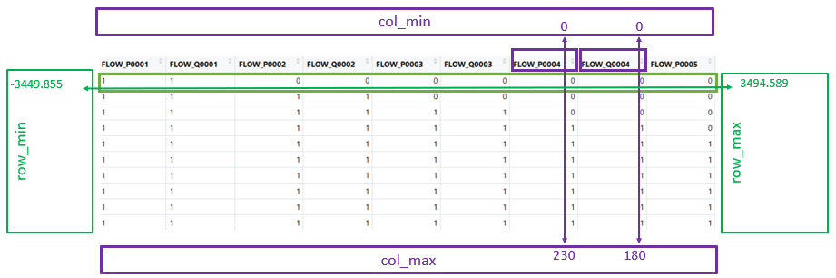
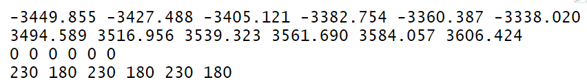
```{r}
# See the example with h=1 about the calculation and division by 3600
row_min <- ( - vol_max +  hydro$INITIAL ) / 3600 + ( hydro$SUPPLY1 + hydro$SUPPLY2 - hydro$LOSS ) 
row_max <- (              hydro$INITIAL ) / 3600 + ( hydro$SUPPLY1 + hydro$SUPPLY2 - hydro$LOSS ) 

col_min <- rep(0, times = (2*hours))
col_max <-  rep(c(230,180), times = hours)


head(row_min)
head(row_max)
head(col_min)
head(col_max)
```

The 4 boundaries have been created as four vectors:

---

The revenue function to maximize

We need to build the vector « revenue » which is representing the function of optimize.

This is the sum of turbine p and turbine q, each hour, indeed the sum of all variables multiplied with the pricing coefficient.

In our use case, it can be schematized with:

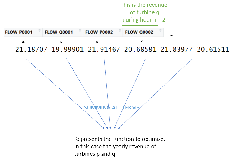
```{r}
# revenues to maximize: 
revenue_turbine_p <-  hydro$COEF_P * hydro$SPOT_PRICE_P 
revenue_turbine_q <-  hydro$COEF_Q * hydro$SPOT_PRICE_Q 
revenue <- as.vector(rbind(revenue_turbine_p, revenue_turbine_q))
head(revenue)
```

The head of the vector « revenue » is:

---

Preparation of the possible error messages

```{r}
# Error messages list preparation
mip_status <- function(status_code) {
  if (status_code == "optimal") {
    cat("Proven Optimal")
  } else if (status_code == "unbounded") {
    cat("Proven Dual Infeasible")
  } else if (status_code == "infeasible") {
    cat("Proven Infeasible")
  } else if (status_code == "nodelimit") {
    cat("Node Limit Reached")
  } else if (status_code == "solutionlimit") {
    cat("Solution Limit Reached")
  } else if (status_code == "abandoned") {
    cat("Abandoned")
  } else if (status_code == "iterationlimit") {
    cat("Iteration Limit Reached")
  } else if (status_code == "timelimit") {
    cat("Seconds Limit Reached")
  } else if (status_code == "unknown") {
    cat("Unknown")
  } else {
    cat("Status unknown")
  }
}

---

Launch of Simplex algorithm

system.time({
  status_code <- cbc_solve(obj = revenue,
                           mat = matrice,
                           is_integer = rep(FALSE, times = (2*hours)),
                           row_lb = row_min,
                           row_ub = row_max,
                           col_lb = col_min,
                           col_ub = col_max,
                           max = TRUE,
                           cbc_args = list(sec = 3600,
                                           PassP = 10))
})

We have an answer after 27 seconds, with a laptop :

---

Checking the status of the simplex:

```{r}
mip_status(solution_status(status_code))
```

Simplex indicates it has found a solution:

---

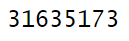
Checking the objective, which is the revenue in EUR

```{r}
objective_value(status_code)
```

The revenue is 31.6 million €:

---

Displaying the variables solution

```{r}
column_solution(status_code)
```

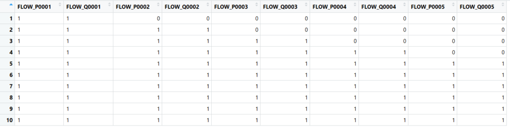
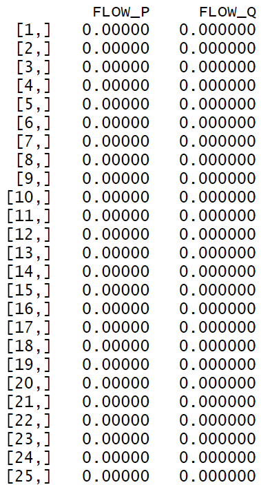
The first page is:

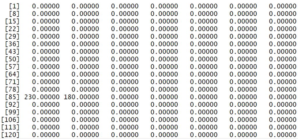
The display as interlaced flow_p and flow_q is not visual enough:

---

Arranging the variables solution display

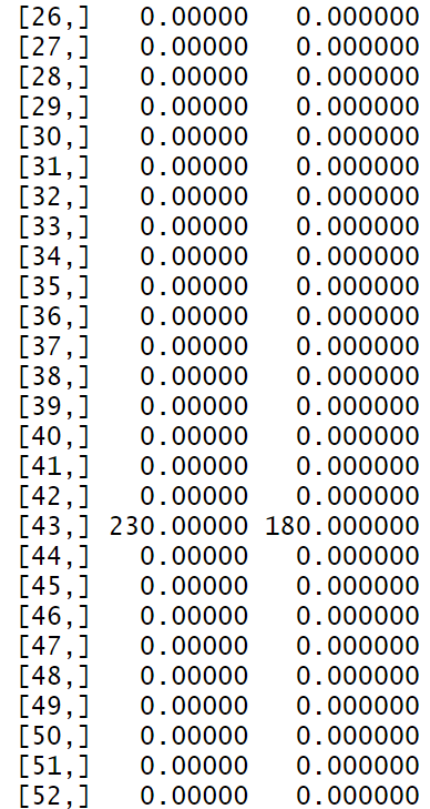
```{r}
solution <- matrix(column_solution(status_code), nrow = hours, ncol = 2, byrow=TRUE)
colnames(solution) <- c("FLOW_P", "FLOW_Q")
print(solution)
```

You can see a small extract of the two turbines flows:

Uploading the solution file

```{r}
dtsolution <- setDT(as.data.frame(solution))
write.table(dtsolution, file = 'C:\\Users\\vincent\\...\\solution.csv', sep =';', row.names = FALSE, col.names = TRUE)
```

---

Business analysis of the solution

The first step is to check if the result is realistic in order to remove any flagrant mistakes. The yearly revenue of 31.6 million euros seems correct:

• 31.6 billion euros would have been definitely incorrect
• 31.6 euros would have been definitely incorrect
• – 31.6 million euros would have been definitely incorrect

Indeed, in a company use case, you are able to check with business team:

• comparing with revenues of the previous years
• getting their feedback about your result

Business interpretation of the variables: due to limitation of the water supply, there are few moments for opening the turbines. Thus, the solution is to store water in the reservoir, and to release only when the spot price is maximum.

The turbine p seems used more often than turbine q, due to globally better spot prices and better coefficient of energy transformation

When a turbine is open, it is usually at full throttle: for full benefit of the high spot price

---

Additional checks

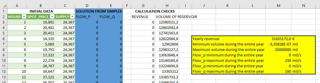
With Excel and with some formulas we are checking if all constraints are ok, if the optimum can retrieved, and how the volume is evolving with time:

Everything is fine, just note the rounding effet -3.E-07 meaning -0.0000003

---

The conclusion from Return On Investment point of view of the Hydropower example

Before this Simplex application, the company knew its hydropower yearly planning was not optimal, as the calculations are done with Excel and iterations.

Not knowing the optimal solution, means that it doesn’t know how close it is from him: maybe it is 80%, 95% or 99% of the optimal solution.

The optimal solution is 31.6 million EUR per year

It means that between the previous solution, and the optimal solution, each 1% gap means 0.32 million EUR per year:

• if the previous solution was 99% close to optimal solution, the company will have a benefit of 0.32 M EUR each new year
• if the previous solution was 90% close to optimal solution, the company will have a benefit of 3.2 M EUR each new year

---

The conclusion from Simplex algorithm point of view

With Simplex algorithm, remember:

As it was a linear problem

• we found a solution
• indeed, we found the best solution
• the solution was quick to find

---

References

Initial Problem described in:

A. Nakib, E-G. Talbi, A. Fuser, « A Hybrid metaheuristic for annual hydropower generation, » In Proc. Of the 28th IEEE Int. Parallel and Distributed Processing Symposium, IPDPS’2014, pp. 747-481, Phoenix, AZ, USA, May 19-23, 2014.