Disclaimer
Even If you know the card game SET, reading the next paragraph could also be informational because it includes the terminology which will be used in R programming, and it reminds the 81 possible cards.

Introduction of the card game SET
This paragraph is quoted from Wikipedia, https://en.wikipedia.org/wiki/Set_(card_game), describes the game and focuses on the definition of a set in the game SET
Set (stylized as SET) is a real-time card game designed by Marsha Falco in 1974 and published by Set Enterprises in 1991. The deck consists of 81 unique cards that vary in four features across three possibilities for each kind of feature: number of shapes (one, two, or three), shape (diamond, squiggle, oval), shading (solid, striped, or open), and color (red, green, or purple).[1] Each possible combination of features (e.g. a card with three striped green diamonds) appears as a card precisely once in the deck.
In the game, certain combinations of three cards are said to make up a set. For each one of the four categories of features — color, number, shape, and shading — the three cards must display that feature as a) either all the same or b) all different. Put another way: For each feature, the three cards must avoid having two cards showing one version of the feature and the remaining card showing a different version.
For example, 3 solid red diamonds, 2 solid green squiggles, and 1 solid purple oval form a set, because the shadings of the three cards are all the same, while the numbers, the colors, and the shapes among the three cards are all different.
For any « set », the number of features that are all the same and the number of features that are all different may break down as 0 the same + 4 different; or 1 the same + 3 different; or 2 the same + 2 different; or 3 the same + 1 different. (It cannot break down as 4 features the same + 0 different as the cards would be identical, and there are no identical cards in the Set deck.)
By Miles, at English Wikipedia The designs are copyrighted by Marsha J. Falco, but I am claiming fair use for the article about Set. I created the image of the physical cards using Adobe Photoshop 6.0, and released my contributions to this image into the public domain. https://commons.wikimedia.org/w/index.php?curid=41704461

By Cmglee – Own work, CC BY-SA 4.0, https://commons.wikimedia.org/w/index.php?curid=66776401
The rulebook in English: https://www.setgame.com/sites/default/files/instructions/SET%20INSTRUCTIONS%20-%20ENGLISH.pdf
The rulebook in French: https://www.gigamic.com/files/catalog/products/rules/gigamic_jset_set_rules.pdf
You can also watch this video tutorial:
The initial context of this post
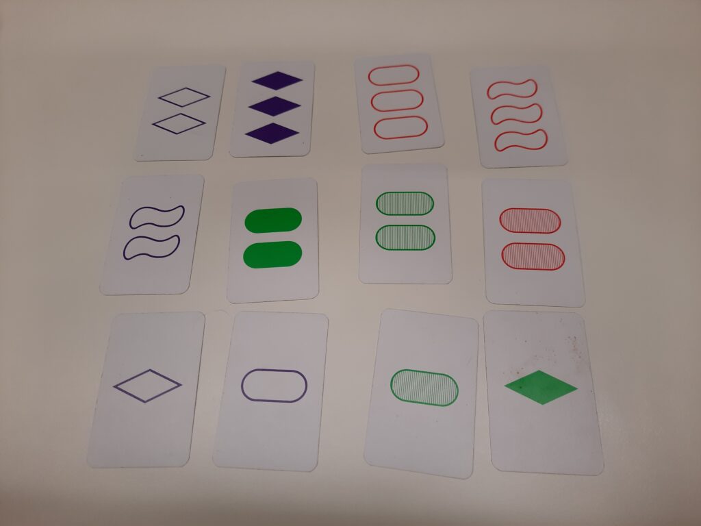
Two players, absolute beginners to this game, including the writer of this post, didn’t find a set in this 12-cards enigma deck:
Courtesy of Laurent Monchy
The owners and experts of the game also didn’t find a set.
Is it sure there is no solution?
The aim of this page
The objectives are:
- This post: is there a set in the focused picture? is there always a set amongst 12 cards?
- The next post: can we estimate the probability of getting a set amongst 12 cards?
Is there always a set in the enigma picture?
Courtesy of Laurent Monchy
Terminology
We will keep the Wikipedia terminology, which will be a bridge between the player world and the R language world.
The possible colors are:
- green
- purple
- red
The possible numbers are:
- One
- Two
- Three
The possible shades are:
- Ppen
- Striped
- Solid
The possible symbols are:
- Diamond
- Squiggle
- Oval
We have chosen an alphabetical sorting for the 4 features and now will always keep it:
COLOR / NUMBER / SHADE / SYMBOL
For instance, consider this card:
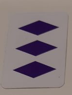
Courtesy of Laurent Monchy
Remember we will program with R language. The first step is to modelize this 12-card deck into data.table
Modelization of the 12-card deck in R language
First, we need to declare the data.table library:
```{r}
library(data.table)
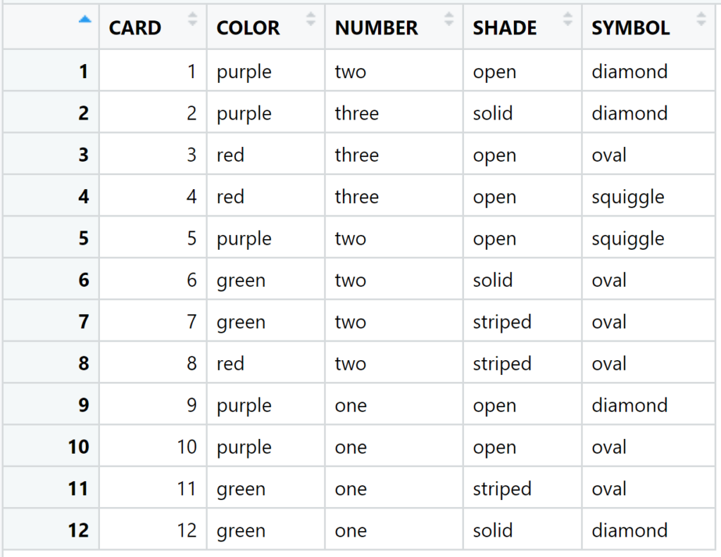
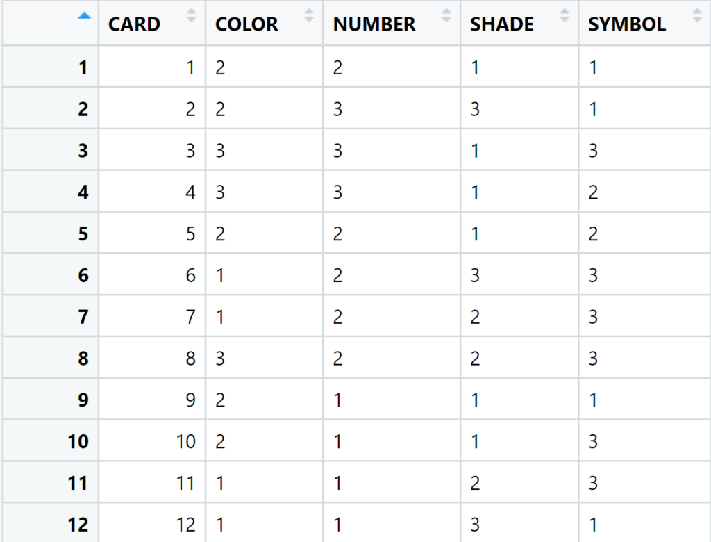
```We create the data.table defining these 12 cards in the enigma picture:
```{r}
# we define the data.table dt_enigma, for which we are looking for a set
dt_enigma <- data.table(CARD=1:12,
                        COLOR  = c("purple", "purple", "red", "red",
                                    "purple", "green", "green", "red",
                                    "purple", "purple", "green", "green" ),
                        NUMBER = c("two", "three", "three", "three",
                                    "two", "two", "two", "two",
                                    "one", "one", "one", "one"),
                        SHADE   = c("open", "solid", "open", "open",
                                    "open", "solid", "striped", "striped",
                                    "open", "open", "striped", "solid"),
                        SYMBOL  = c("diamond", "diamond", "oval", "squiggle",
                                    "squiggle", "oval", "oval", "oval",
                                    "diamond", "oval", "oval", "diamond")
                        )
```
The content of dt_enigma:
We could continue to program with full-text features. Indeed, it will be easier to deal with numbers.
Every triplet of three values is mapped to the values 1, 2, and 3. They are not arbitrary, we’ll explain afterward.
First, we map the features:
| Full-text feature | Numeric feature |
| red | 1 |
| green | 2 |
| purple | 3 |
| Full-text feature | Numeric feature |
| one | 1 |
| two | 2 |
| three | 3 |
| Full-text feature | Numeric feature |
| open | 1 |
| striped | 2 |
| solid | 3 |
| Full-text feature | Numeric feature |
| diamond | 1 |
| squiggle | 2 |
| oval | 3 |
```{r}
# We define 4 lookup data.tables, one for each feature
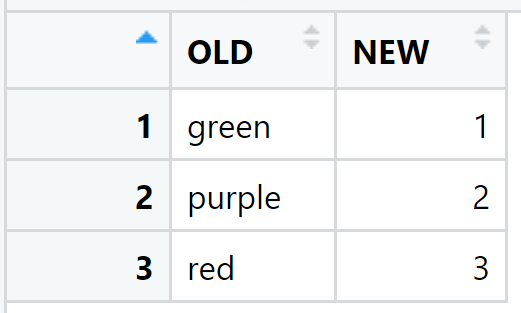
dt_lookup_color <- data.table(OLD = c("green","purple","red"), NEW = c(1,2,3) )
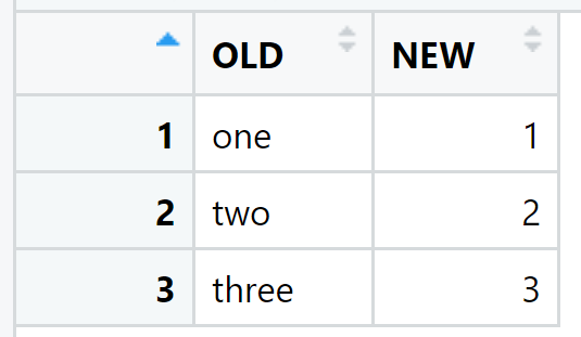
dt_lookup_number <- data.table(OLD = c("one","two","three"), NEW = c(1,2,3) )
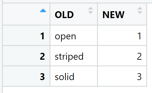
dt_lookup_shade <- data.table(OLD = c("open","striped","solid"), NEW = c(1,2,3) )
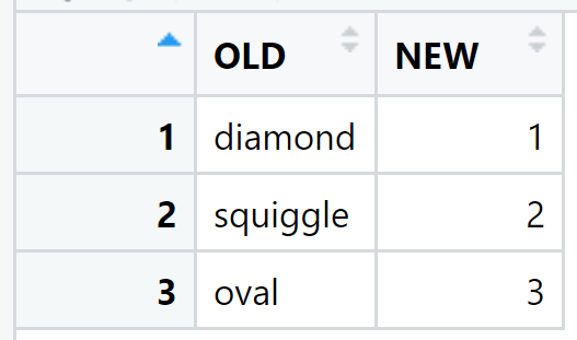
dt_lookup_symbol <- data.table(OLD = c("diamond","squiggle","oval"), NEW = c(1,2,3) )
```The content of dt_lookup_color:
The content of dt_lookup_number:
The content of dt_lookup_shade:
The content of dt_lookup_symbol:
```{r}
# For each feature, we replace the full-text by its numeric
# We indicate 1 the working data.table dt_enigma
#             2 the lookup data.table to be searched
#             3 the starting working column
#             4 the starting lookup column
#             5 the destination working column
#             6 the destination lookup column
#
#            1          2                     3       4     5          6
dt_enigma <- dt_enigma[ dt_lookup_color, on=.(COLOR = OLD), COLOR := i.NEW]
dt_enigma <- dt_enigma[ dt_lookup_number, on=.(NUMBER = OLD), NUMBER := i.NEW]
dt_enigma <- dt_enigma[ dt_lookup_shade, on=.(SHADE = OLD), SHADE := i.NEW]
dt_enigma <- dt_enigma[ dt_lookup_symbol, on=.(SYMBOL = OLD), SYMBOL := i.NEW]
```
The new content of dt_enigma:
Modelization of all the possible 3-card combination
How many combinations of 3 cards are possible with an initial deck of 12 cards?
This is a combination theme: https://en.wikipedia.org/wiki/Combination
The formula is, quoting Wikipedia:
In mathematics, a combination is a selection of items from a collection, such that the order of selection does not matter (unlike permutations). For example, given three fruits, say an apple, an orange, and a pear, three combinations of two can be drawn from this set: an apple and a pear; an apple and an orange; or a pear and an orange. More formally, a k-combination of a set S is a subset of k distinct elements of S. If the set has n elements, the number of k-combinations is equal to the binomial coefficient
which can be written using factorials as

whenever k ≤ n, and which is zero when k > n.
We define a small function in R to calculate it:
# A small function for calculating the combination
my.combination = function(n, k) {
  factorial(n) / factorial(n-k) / factorial(k)
}
We call it for n = 12 cards, k = 3 cards, as we are looking for the total number of combinations of 3 cards amongst 12 cards
```{r}
my.combination(81,3)
```
Hence, we have good news: the number of combinations is reasonable, and we will calculate all of them.
In R language, the combined function allows to generation all the solutions in a matrix format.
```{r}
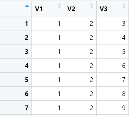
# We create a matrix with all combinations of 3 cards within 12
mt_combination <- combn( seq(1,12,1), 3 )
# We prefer to transpose and each combination switch from column to row
mt_combination <- t(mt_combination)
# We convert into data.frame, intermediary
df_combination <- as.data.frame(mt_combination)
# We convert into data.frame, the target
dt_combination <- setDT(df_combination)
# We rename the columns
colnames(dt_combination) <- c("CARD1", "CARD2", "CARD3")
```We will download for the purpose of the post:
```{r}
write.csv2(dt_combination, file = "C:/Users/vince/Downloads/ dt_combination.csv")
```
We can have a look at the first entries of the combination:
Gathering the features of all the 220 triplets
As we have found the 220 triplets, we need to fetch the 4 features of each component, in order to compare them and to determine the set eligibility.
For any « set », the number of features that are all the same and the number of features that are all different may break down as 0 the same + 4 different; or 1 the same + 3 different; or 2 the same + 2 different; or 3 the same + 1 different.
A reminder from https://en.wikipedia.org/wiki/Set_(card_game)
```{r}
# We remind the columns names of the enigma
colnames(dt_enigma)
```
```{r}
# We remind the columns names of the combination
colnames(dt_combination)
```
It is time to merge, or inner-join if you get used to SQL
Remark: as the same procedure is applied 3 times, it could have been automatized in a function. Let’s be foolish and abuse copy-paste
```{r}
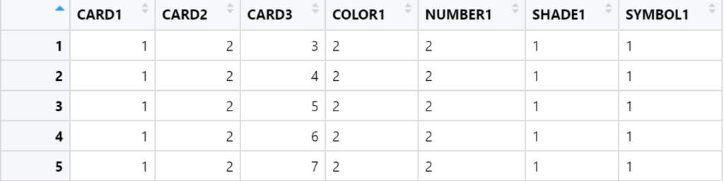
# We need to have relevant features names for the first card of the combination
colnames(dt_enigma) <- c("CARD", "COLOR1", "NUMBER1", "SHADE1","SYMBOL1")
# We merge, indeed inner join, the combination with the columns of the first card
dt_fulldata <- merge( dt_combination, dt_enigma, by.x = "CARD1", by.y = "CARD")
```
```{r}
# We need to have relevant property names for the second card of the combination
colnames(dt_enigma) <- c("CARD", "COLOR2", "NUMBER2", "SHADE2","SYMBOL2")
# We merge, indeed inner join, the combination with the columns of the second card
dt_fulldata <- merge( dt_combination, dt_enigma, by.x = "CARD2", by.y = "CARD")
```
```{r}
# We need to have relevant property names for the second card of the combination
colnames(dt_enigma) <- c("CARD", "COLOR3", "NUMBER3", "SHADE3","SYMBOL3")
# We merge, indeed inner join, the combination with the columns of the second card
#  note the difference↓↓↓↓↓↓↓↓↓↓↓ , as we complete dt_fulldata
dt_fulldata <- merge( dt_fulldata, dt_enigma, by.x = "CARD3", by.y = "CARD")
```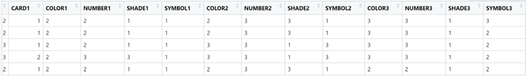
We reorder the columns, to be able to visualize and compare the same properties of triplet:
```{r}
# Reorder the columns, for clarity: grouped by features type
setcolorder(dt_fulldata, neworder =c("CARD1" , "CARD2", "CARD3",
                                  "COLOR1", "COLOR2", "COLOR3",
                                  "NUMBER1", "NUMBER2", "NUMBER3",
                                  "SHADE1", "SHADE2", "SHADE3",
                                  "SYMBOL1", "SYMBOL2", "SYMBOL3"
                                  ) )
```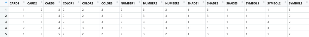
Checking if the row is a set or not
As promised, let’s see why we have chosen 1, 2, and 3 as numeric values defining the four feature values.
Case 1: if the 3 values of a feature are all 3 the same
There are 3 possibilities: 1/1/1, 2/2/2 and 3/3/3
If you sum the 3 values, it provides respectfully : 3, 6, and 9
Remind the modulo operation?
In mathematics, the modulo operation works out the remainder (what’s left over) when we divide two integers (whole numbers without a fraction or a decimal) together.
For example, 5 modulo 2 is 1, because if we divide 5 by 2, then we get 2 (because 2 × 2 = 4 ) with 1 left over. Instead of writing modulo, people sometimes write mod
Quoted from https://simple.wikipedia.org/wiki/Modulo_operation
In R language, the modulo operator is %%. Some examples with modulo 3:

We return to the resolution of case 1.
If you sum the 3 values, it provides respectfully : 3, 6, and 9
The corollary is :
If you sum the 3 values and apply modulo 3 to the sum, it provides: 0, 0, 0 when the three features are the same as 3 modulo 3 = 0 / 6 modulo 3 = 0, 9 modulo 3 = 0.
Case 2: if the 3 values of a feature are all 3 different
There are 6 possibilities: 1/2/3, 1/3/2, 2/1/3, 2/3/1, 3/1/2, 3/2/1
If you sum the 3 values, it provides only: 6
If you sum the 3 values and apply modulo 3 to the sum, it provides: only 0 when the three features are all different as 6 modulo 3 = 0
Case 3: if the 3 features are not all different or not all different
Guess what?
If you sum the three values, which are not all the same or not all different, and apply a modulo, the value will be different from zero.
The result will be always 1 or 2.
For instance:
1/1/3 -> the sum is 5 -> applying modulo 3 -> the result is 2
2/2/3 -> the sum is 7 -> applying modulo 3 -> the result is 1
2/3/3 -> the sum is 8 -> applying modulo -> the result is 2
You can check the other combinations…
Summary of the 3 cases
If the 3 values of one feature for 3 cards are all equal or all different: the « sum modulo 3 » is equal to 0.
If the 3 values of one feature for 3 cards are not all equal and not all different: the « sum modulo 3 » is not equal to 0.
We have now a quick way to determine if the feature is relevant or not for a set
Application of sum modulo 3 in R programming
We create 4 new columns which are the « sums modulo 3 » as explained above:
```{r}
# Copy the working data.table as safety
dt_checkset <- copy(dt_fulldata)
# Oops, the features had kept the CHARACTER from the full text feature. We need to switch to NUMERIC
columns_require_num <- c("COLOR1", "COLOR2", "COLOR3" ,
                 "NUMBER1", "NUMBER2", "NUMBER3",
                 "SHADE1",  "SHADE2",  "SHADE3",
                 "SYMBOL1", "SYMBOL2", "SYMBOL3"
                 )
# Convert the required columns as numeric
dt_checkset[, (columns_require_num) := lapply(.SD, as.numeric), .SDcols = columns_require_num]
# Each feature gets a sum column + a modulo 3
dt_checkset[, SUM_COLOR := ( COLOR1 + COLOR2 + COLOR3 ) %% 3 ]
dt_checkset[, SUM_NUMBER := ( NUMBER1 + NUMBER2 + NUMBER3 ) %% 3 ]
dt_checkset[, SUM_SHADE := ( SHADE1 + SHADE2 + SHADE3 ) %% 3 ]
dt_checkset[, SUM_SYMBOL := ( SYMBOL1 + SYMBOL2 + SYMBOL3 ) %% 3 ]
```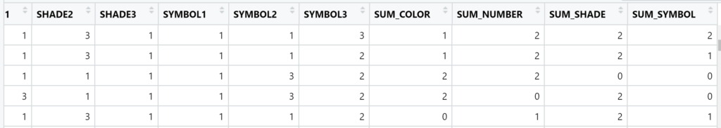
A triplet is a set, if, for each feature, the values are all the same or different.
Hence a triplet is a set, if all sums with modulo 3 are equal to 0
It implies that a triplet is a set if the sum of the four « sums with modulo 3 » is equal to zero, because 0 + 0 + 0 + 0 = 0
```{r}
# If the value in column SET_CHECK is zero, it means it is a set
dt_checkset[, SET_CHECK := SUM_COLOR + SUM_NUMBER + SUM_SHADE + SUM_SYMBOL ]
# Generate an Excel file
write.csv2(dt_checkset, file = "C:/Users/vince/Downloads/dt_checkset.csv")
```
Hereunder the generated .csv file:
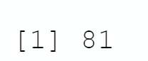
We want to know if there is a set in the Enigma picture!
```{r}
# How many rows with the value of column SET_CHECK equal to zero?
number_of_set <- nrow(dt_checkset[SET_CHECK == 0])
print(number_of_set)
```
This 12-card deck contains no set! The players and the owners were right!
Conclusion of the question « Does every 12-card combination have at least one solution? «
No, some combination, may be without any set. The game rule explains how to move on.
Each day you can try to find one SET:
https://www.setgame.com/set/puzzle
Or, better, you could purchase the physical game

What is the probability of not finding a set among 12 cards
R-language program
The first step in the R program is to declare the packages
```{r}
# We will use data tables
library(data.table)
# We will graphically check the convergence of probability
library(ggplot2)
```
We create in a data.table all the 81 cards of the game SET, knowing all the different combinations of 3 colors, 3 numbers, 3 shades and 3 symbols are displayed
```{r}
# We define all the 81 cards of the set game
COLOR  <- c(1,2,3) #all the possibilities of colors encoded, respectively "green","purple","red"
NUMBER <- c(1,2,3) #all the possibilities of colors encoded, respectively "one","two","three"
SHADE  <- c(1,2,3) #all the possibilities of colors encoded, respectively "open","striped","solid"
SYMBOL <- c(1,2,3) #all the possibilities of colors encoded, respectively "diamond","squiggle","oval"
all_cards <- expand.grid( COLOR = COLOR,
                          NUMBER = NUMBER,
                          SHADE = SHADE,
                          SYMBOL = SYMBOL
                          )
all_cards <- setDT(all_cards)
# Check 81 cards are generated
print(nrow(all_cards))
```
We are checking the 81 cards:
```{r}
write.csv2(all_cards, file = "C:/Users/vince/Downloads/all_cards.csv")
```
The data.table all-cards is:
Many code lines from the previous post are gathered in order to create a function is_set:
- In the entry parameter: a data.table containing an undetermined number of cards. The columns in data.table must be in the format of the above file
- Out the return parameter: 1 if there is at least one set, 0 if no set at all
Remark: the 12 cards are chosen randomly amongst all 81 cards
We’ll detail this at the end of the post
```{r}
is_set <- function(dt_enigma) {
# We create a matrix with all combinations of 3 cards within 12
mt_combination <- combn( seq(1,12,1), 3 )
# We prefer to transpose and each combination switch from column to row
mt_combination <- t(mt_combination)
# We convert into data.frame, intermediary
df_combination <- as.data.frame(mt_combination)
# We convert into data.frame, the target
dt_combination <- setDT(df_combination)
# We rename the columns
colnames(dt_combination) <- c("CARD1", "CARD2", "CARD3")
# add the ID of card
dt_enigma <- cbind( data.table( CARD = c(1:12)) , dt_enigma)
# We need to have relevant property names for the first card of the combination
colnames(dt_enigma) <- c("CARD", "COLOR1", "NUMBER1", "SHADE1","SYMBOL1")
# We merge, indeed inner join, the combination with the columns of the first card
dt_fulldata <- merge( dt_combination, dt_enigma, by.x = "CARD1", by.y = "CARD")
# We need to have relevant property names for the second card of the combination
colnames(dt_enigma) <- c("CARD", "COLOR2", "NUMBER2", "SHADE2","SYMBOL2")
# We merge, indeed inner join, the combination with the columns of the second card
# note the difference↓↓↓↓↓↓↓↓↓↓↓ , as we complete dt_fulldata
dt_fulldata <- merge( dt_fulldata, dt_enigma, by.x = "CARD2", by.y = "CARD")
# We need to have relevant property names for the second card of the combination
colnames(dt_enigma) <- c("CARD", "COLOR3", "NUMBER3", "SHADE3","SYMBOL3")
# We merge, indeed inner join, the combination with the columns of the second card
# note the difference↓↓↓↓↓↓↓↓↓↓↓ , as we complete dt_fulldata
dt_fulldata <- merge( dt_fulldata, dt_enigma, by.x = "CARD3", by.y = "CARD")
# Reorder the columns, for clarity: grouped by property type
setcolorder(dt_fulldata, neworder =c("CARD1" , "CARD2", "CARD3",
"COLOR1", "COLOR2", "COLOR3",
"NUMBER1", "NUMBER2", "NUMBER3",
"SHADE1", "SHADE2", "SHADE3",
"SYMBOL1", "SYMBOL2", "SYMBOL3"
) )
# Copy the working data.table as safety
dt_checkset <- copy(dt_fulldata)
# Oops, the features had kept the CHARACTER format from the full text feature. We need to switch to NUMERIC
columns_require_num <- c("COLOR1", "COLOR2", "COLOR3" ,
"NUMBER1", "NUMBER2", "NUMBER3",
"SHADE1", "SHADE2", "SHADE3",
"SYMBOL1", "SYMBOL2", "SYMBOL3"
)
# Convert the required columns as numeric
dt_checkset[, (columns_require_num) := lapply(.SD, as.numeric), .SDcols = columns_require_num]
# Each feature gets a sum column + a modulo 3
dt_checkset[, SUM_COLOR := ( COLOR1 + COLOR2 + COLOR3 ) %% 3 ]
dt_checkset[, SUM_NUMBER := ( NUMBER1 + NUMBER2 + NUMBER3 ) %% 3 ]
dt_checkset[, SUM_SHADE := ( SHADE1 + SHADE2 + SHADE3 ) %% 3 ]
dt_checkset[, SUM_SYMBOL := ( SYMBOL1 + SYMBOL2 + SYMBOL3 ) %% 3 ]
# If the value in column SET_CHECK is zero, it means it is a set
dt_checkset[, SET_CHECK := SUM_COLOR + SUM_NUMBER + SUM_SHADE + SUM_SYMBOL ]
number_of_sets <- nrow(dt_checkset[, dt_checkset[SET_CHECK == 0] ])
# We translate the numeric into boolean: if TRUE, this is a set
if (number_of_sets == 0) {result_boolean <- 0 } else { result_boolean <- 1 }
return( result_boolean )
}
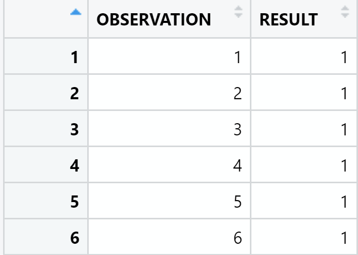
```Let’s test with 100 samples of 12 cards: as a result, the number of sets should be close but smaller than 100, as we know « no set » is uncommon
Remark: every time we run the program, the function set.seed allows us to initialize the random number sequence using the provided seed. Otherwise, the random number sequence is not reproducible.
```{r}
set.seed(1)
counter <- 0
for (i in 1:100 ) {
petit_test <- all_cards[sample(nrow(all_cards), 12, replace = FALSE),  ]
counter <- counter + is_set(petit_test)
}
print(counter)
```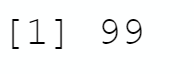
We change the parameter value provided to set.seed from 0 to 3, in order to check if the result is different:
```{r}
set.seed(3)
counter <- 0
for (i in 1:100 ) {
petit_test <- all_cards[sample(nrow(all_cards), 12, replace = FALSE),  ]
counter <- counter + is_set(petit_test)
}
print(counter)
```
With these two experiences, each with 100 observations, we have two results that seem consistent: 1% and 5% of none-set
The corollary questions are:
- When increasing the number of observations, will the probability converge as expected?
- Will the probability found be precise?
A function is_set is created, for mass testing the existence of sets:
- In, the first entry parameter: the number of observations, indeed the total trials
- Out, the return parameter: a data.table with 2 columns: first the ID of the trial, second the result, 1 is there is a set, 0 if not set
```{r}
generate <- function(nb_observations) {
  # We want to have reproducible observations
  set.seed(1)
  # We sample nb_observations of nb_cards cards
  # A selected card cannot be generated again, so we don't replace the cards, hence replace = FALSE
  for (i in 1:nb_observations) {
    i_draw <- all_cards[sample(nrow(all_cards), 12, replace = FALSE),  ]
    i_result <- is_set(i_draw)
    if (i  == 1) {
      row_result <- data.table( OBSERVATION = c(i), RESULT = c(i_result) )
    } else {
      l = list(row_result , data.table( OBSERVATION = c(i), RESULT = c(i_result) ) )
      row_result <- rbindlist( l )
    }
  }
  return(row_result)
}
```
The code for running 1.000.000 observations of 12 cards: as it should need a couple of hours, you may want to try first with fewer observations:
my_sample <- generate(1000)my_sample <- generate(10000)my_sample <- generate(100000)You can run yourself the previous codes, on this post, we will focus on 1.000.000 observations:
my_sample <- generate(1000000)An extract of my_sample:
Find hereunder the content of my_sample, 18 MB:
```{r}
write.csv2(my_sample, file = "C:/Users/vince/Downloads/my_sample.csv")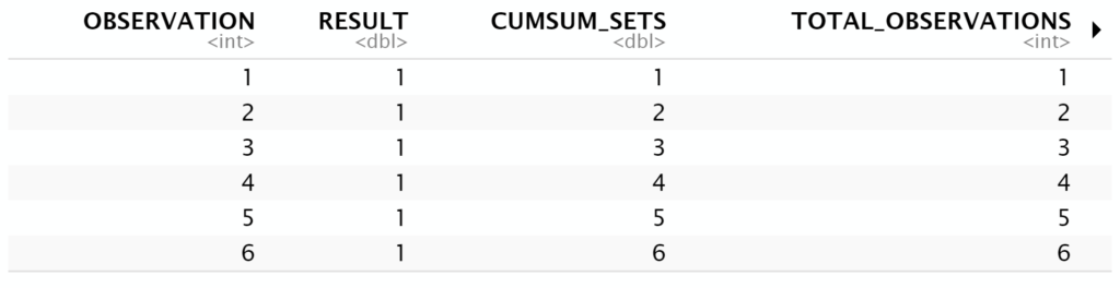
```Now we want to determine the evolution of the global percentage set compared to the number of observations:
```{r}
my_sample <- my_sample[ , CUMSUM_SETS := cumsum(RESULT)]
my_sample <- my_sample[ , TOTAL_OBSERVATIONS  := .I ]
my_sample <- my_sample[ , GLOBAL_PERCENTAGE_SET  := CUMSUM_SETS / OBSERVATION ]
```
An extract of my_sample:
```{r}
head(my_sample)
```

The main question, in order to check if the program approach is correct: is there a convergence of the global probabilities?
We plot the result
```{r}
my_plot <- ggplot(my_sample, aes(x=OBSERVATION, y=GLOBAL_PERCENTAGE_SET))
my_plot + geom_line() + ggtitle("Evolution of probability with observations") + ylab("Global percentage of set founds") + xlab("Number of observations")
```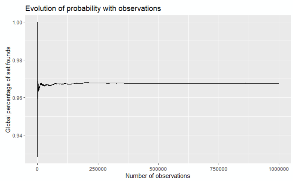
We graphically assume the series is converging.
Hence we can consider the global estimation with 1000000 observations is an estimation of the probability of « finding a set amongst 12 cards »
```{r}
# Get the last row
last_row <- tail(my_sample,1)
# Extract the global percentage
probability_of_set <- last_row[1,"GLOBAL_PERCENTAGE_SET"]
print(probability_of_set)
```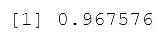
```{r}
probability_of_no_set <- 1 - probability_of_set
print(probability_of_no_set)
```
The probability of not finding a set is 3.24%
Evolution of the probability during the life of game
When the author of this post met this scenario, it was in the middle of a game :
Do you remember this previous remark?
Remark: the 12 cards are chosen randomly amongst all 81 cards
We’ll detail this at the end of the post
It had been coded with this code line:
i_draw <- all_cards[sample(nrow(all_cards), 12, replace = FALSE), ]As the 12 cards have been chosen amongst 81 cards, it means the previous calculations were done during the first round, in this configuration:
At the beginning of the game, 12 cards are fetched from the draw of 81-cards and become the deck
It may not be obvious, but the probability of finding a set is evolving during the game.
It won’t be studied in this post, nevertheless, some leads are provided, in case you want to study the evolution of probabilities during the game.
It would be required to develop full SET game behavior.
A python language example is available:
https://github.com/aloverso/setgame
Bad luck, it has been developed with Python language.
Another lead, Peter Norvig has compared the 2 following scenarios:
- The probability of a none-set at the beginning of the game: around 3.3% with 100.000 observations: to be compared with our 3.24% with 1.000.000 observations.
- The probability of a none-set during the entire game: around 5.7%
Remark – the difference 3.3% datascience.lc VS 3.24% norvig.com can be explained with:
- With the R program, we had shown a probability of 3.24% with 1.000.000 observations. If you run this program with 100.000 observations or open the file my-sample1.csv, you find out the probability is 3.30%: it means at 100.000 the precision looks like only 1 digit after the decimal point
- The R program is reproducible with the set.seed option, it is unknown in the comparison program, and as the observations should not have been the same: randomness occurs!
Conclusion of the question « What is the probability of not finding a set among 12 cards »
As we had no analytic solution for the probability of « no set », we have chosen the programming simulation option.
A convergence was graphically noticed: subjectively, it is quickly noted, but it is slow if high precision is required.
We have estimated that the probability of no-set, in the first round of the game, is 3.24%.
We have also learned this probability of no-set is evolving during the lifecycle of the game and is g