Introduction
In the 17th century, the astronomer Galileo has noted errors of measurement with his astronomical observations.
These errors were easily explained by the imperfections of the instruments.
Indeed, he has noted :
- The errors are symmetrical
- Small errors occur often than big errors
- The shape of the distribution looks like a smooth curve
These errors looks like this:
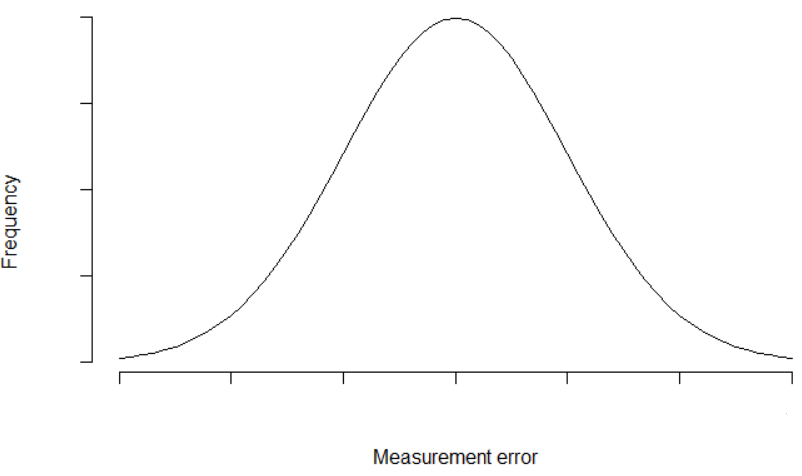
This smooth curve is called « Normal distribution » and is recurring in Nature, for example :
- The weight of tomatoes, before calibration
- The height of women in France, the height of men in France
- The sum of a « considerable number » of dice
Wait a minute
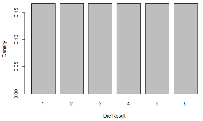
Yes, we mean the sum of a « considerable number » of dice « not loaded, fair » dice: they have the same probability to provide 1, 2, 3, 4, 5, or 6. It’s called a uniform distribution:
And when we sum a » considerable number of » dice, the result would be like hereunder?
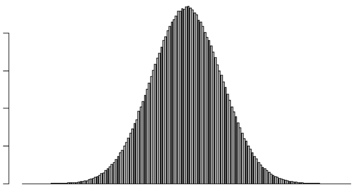
Let’s check it!
R programming: do we really get a normal distribution when summing dices?
The importance of the number of observations in statistics: the study of one-die rolls
The frequency is the number of observations.
The density is the probability: it can be a percentage or a number: for example 8% or 0.08.
Roll one die, 10 times
We kick off easy, in order to warm up with R programming.
We are simulating with the R function sample, the die roll. For example, the function sample(1:6) is used.
Let’s start to simulate 10 rolls:
No library is required. We want to avoid scientific notation in the plots, hence we begin with:
```{r}
# No need of library
options(scipen = 999) # Avoid scientific notation
```
The core of the roll:
```{r}
# Let's run an observation with 10 dices: what is the frequency?
###
# We want to have reproducible observations
set.seed(1)
# We choose to roll 10 times
number_rolls <- 10
# With the sample function, we simulate the rolls; "replace = "TRUE" indicates it's ok to have similar results. For example, if you roll 2 dice, it is possible to get twice the value 1.
observations <- sample(1:6,number_rolls, replace = TRUE)
# We count the results
result <- table(observations)
print(result)
```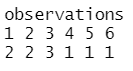
The first row describes the possible value of the die.
The second row describes the frequency according to the values.
In the sample function « replace = « TRUE » indicates it’s ok to have similar results.
For example, if you roll 2 dice, it is possible to get twice the value 1.

« replace = « FALSE » would be used for example when picking numbers from a sphere, but without replacing the numbers after picking, like in lottery Euromillions

Remark: every time we run the program, the function set.seed allows us to initialize the random number sequence using the provided seed. Otherwise, the random number sequence is not reproducible.
Plot the result
```{r}
# We plot the frequency
barplot(result, xlab = "Die Value", ylab = "Frequency")
```
Automatization of the rolls of one die
Let’s create a function for rolling one dice, with number_rolls rolls:
```{r}
# Let's create a function for rolling one dice, with number_rolls rolls
roll_single_die <- function(number_rolls) {
# With the sample function, we simulate the rools; replace = TRUE is a trick indicating it's ok to have one result, for example 1, more than one time
observations <- sample(1:6,number_rolls, replace = TRUE)
# We count the results
result <- table(observations)
barplot(result, xlab = "Die Value", ylab = "Frequency")
}
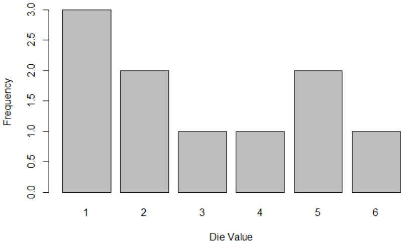
```We can call this function roll_single_die 10 times:
```{r}
roll_single_die(10)
```
The result is not closed to a uniform distribution. Haven’t we stated that the die is fair, unloaded? So increasing the number of observations, we should converge to a uniform distribution.
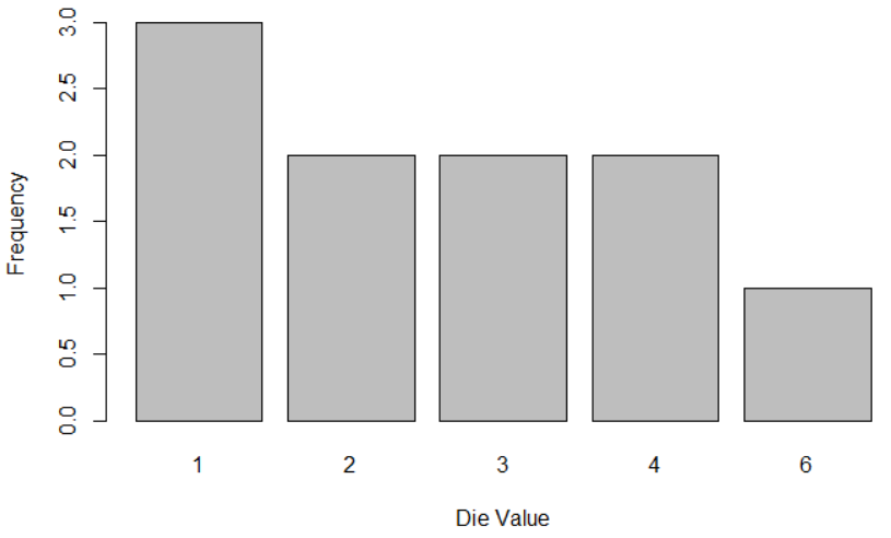
Let’s roll 100 times:
```{r}
roll_single_die(100)
```
It is not obviously converging to a uniform distribution. It’s a little surprising, but it’s Statistics!
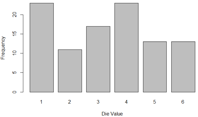
Let’s roll 1000 times:
roll_single_die(1000)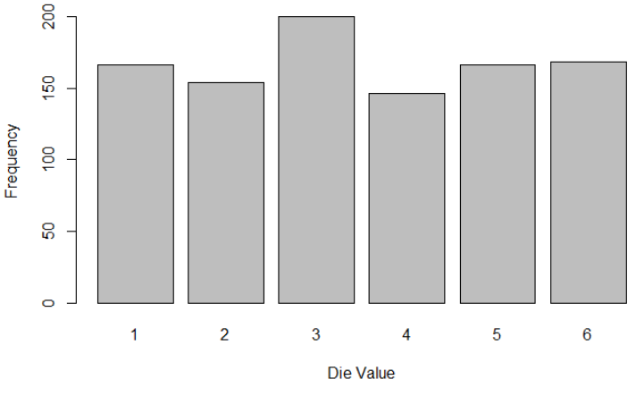
The uniformity is a little better, but not vivid: yes convergence may need a lot of rolls!
Let’s roll 10000 times:
roll_single_die(10000)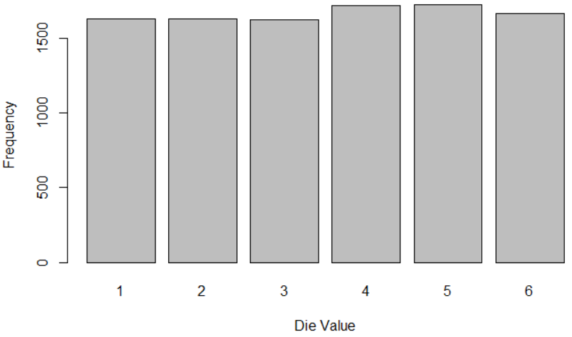
Finally, it is starting to look like a uniform distribution!
One last series of rolls?
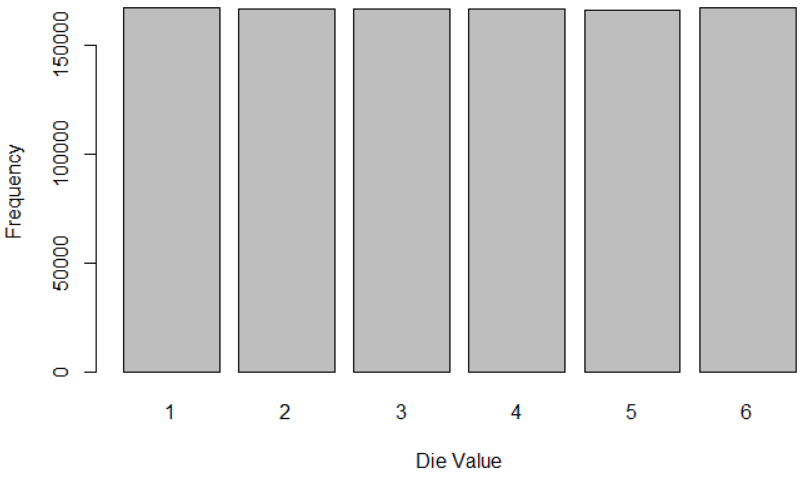
Let’s roll 100000 times:
roll_single_die(100000)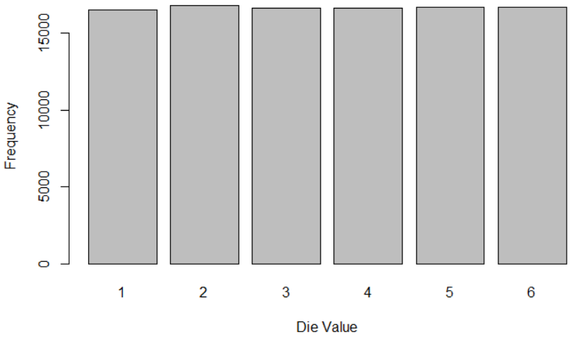
The uniformity is improving.
Let’s roll 1000000 times:
```{r}
roll_single_die(1000000)
```
It looks like a uniform distribution. Nevertheless, we graphically note that the frequencies are close, although not identical: the high number of observations didn’t completely remove the randomness. An even higher number of observations would be required to converge more and more to the uniform distribution.
As a conclusion: we have graphically noted that the simulation is converging to the uniform distribution when the number of dice becomes infinite. And this convergence is subjectively slow and requires a lot of observations!
We arbitrarily assume that our simulator, the « sample » R function is probably random enough with 1000000 rolls for one dice!
For the sum of dice, we will check if roll 1000000 times are enough too.
Study of 2-dice rolls
Now we simulate the rolls of 2 dice and sum the dice values.
```{r}
# Let's run an observation with 2 dices: what is the frequency?
###
# We want to have reproducible observations
set.seed(1)
# We choose to roll 1000000 times
number_rolls <- 1000000
# We choose to sum 2 dices
number_dice <- 2
# With the sample function, we simulate the rools; replace = TRUE is a trick indicating it's ok to have one result, for example 1, more than one time
# We have 10 rolls and 2 dices, hence we need 10*2 = 20 samples
raw_observations <- sample(1:6, number_rolls*number_dice , replace = TRUE)
# We cut the 20 samples, into 10 rolls of 2 dice, meaning a matrix with 10 lines and 2 columns
tidy_observations <- matrix(raw_observations, nrow = number_rolls, ncol = number_dice )
# Remember we sum each roll of 2 dice: we have to create a sum column
sum_observations <- rowSums(tidy_observations)
# We count the results
result <- table(sum_observations)
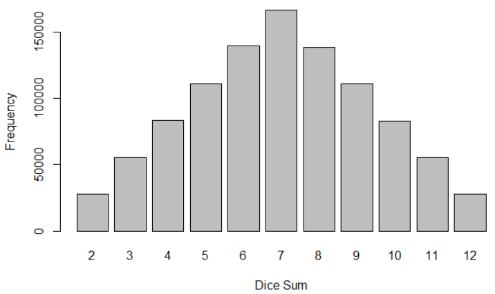
barplot(result, xlab = "Dice Sum", ylab = "Frequency")
```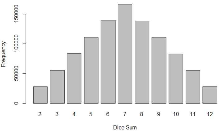
We note that the sum of 2 dice provides a triangle distribution. And you are close to asking me to give you your money back! Hence 2 remarks:
- This site is free of charge
- We have indicated that the sum of « considerable number » of dice will provide a Normal distribution
Let’s increase the number of dice
Automatization of the rolls of numerous dice
We create a function plotting the sum of dice depending on 2 parameters:
- The number of rolls number_rolls
- The number of dice to be summed: number_dice
The function roll_mutiple_dice is created:
```{r}
# Now we are ready to create a function providing the distribution according to:
# The number of rolls: number_rolls
# The number of dice to sum: number_dice
roll_multiple_dice <- function( number_rolls, number_dice ) {
# We want to have reproducible observations
set.seed(1)
# With the sample function, we simulate the rools; replace = TRUE is a trick indicating it's ok to have one result, for example 1, more than one time
# We have number_rolls rolls and number_dice dices, hence we need number_rolls*number_dice  samples
raw_observations <- sample(1:6, number_rolls*number_dice , replace = TRUE)
# We cut the 20 samples, into 10 rolls of 2 dice, meaning a matrix with 10 lines and 2 columns
tidy_observations <- matrix(raw_observations, nrow = number_rolls, ncol = number_dice )
# Remember we sum each roll of 2 dice: we have to create a sum column
sum_observations <- rowSums(tidy_observations)
# We count the results
result <- table(sum_observations)
barplot(result, xlab = "Dice Sum", ylab = "Frequency")
}
```
Roll 1000000 times 2 dice
```{r}
roll_multiple_dice(1000000, 2)
```
You note the reproducibility thanks to the set.seed.
Roll 1000000 times 4 dice
```{r}
roll_multiple_dice(1000000, 4)
```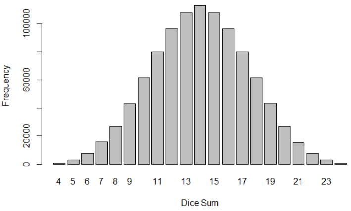
The smoothness curve begins to appear!
Roll 1000000 times 10 dice
```{r}
roll_multiple_dice(1000000, 10)
```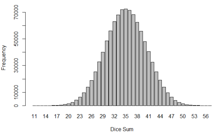
It’s getting better
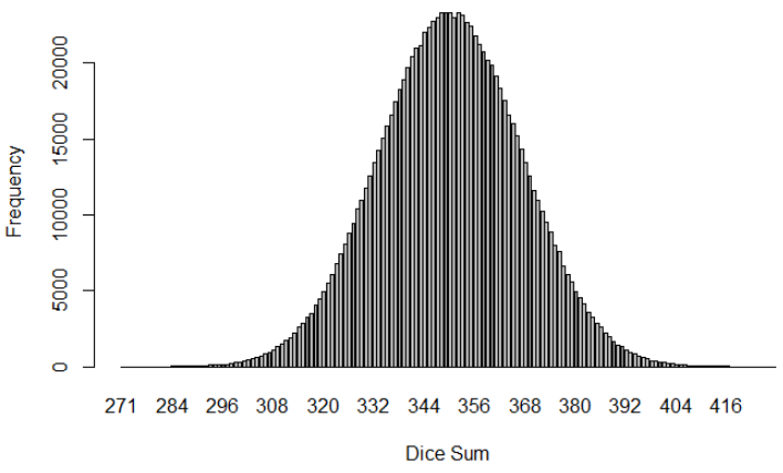
Roll 1000000 times 100 dice
roll_multiple_dice(1000000, 100)
Now it’s graphically clear.
As a summary:
The sum of 100 dice, which have originally a uniform distribution:
Provides a Normal distribution:
This leads us to the Central limit theorem
The Central limit theorem
If you consider:
- a huge and increasing number of random samples
- With independence between these samples (for example, the value of die number 1 is independent of the value of die number 2 when you roll together these two dice, which is also independent of number 3…)
Then their sum is converging to a Normal distribution.
This is a theorem: it means it is proven. And yes, as you guess, the mathematical proof is hairy: https://towardsdatascience.com/central-limit-theorem-proofs-actually-working-through-the-math-a994cd582b33
Let’s be honest, this theorem is like Statistics, counter-intuitive. Hence we are summarizing it with a couple of graphs:
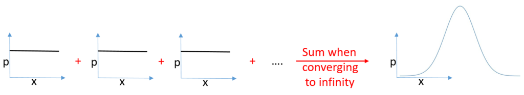
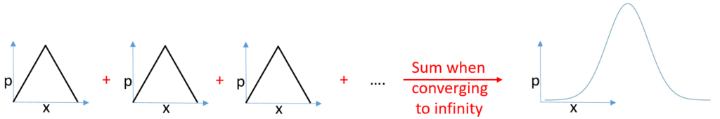
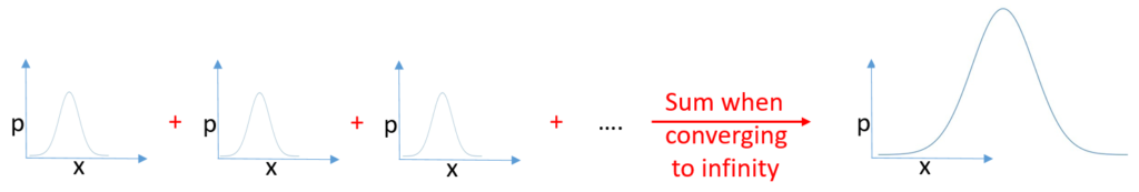
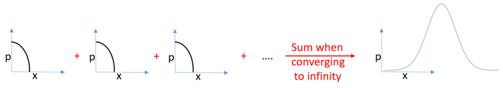
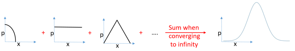
And for whatever sum of distributions, when the number of distributions is converging to infinity. Don’t forget the distributions must be independent.
Application of the Central Limit Theorem to the weight of tomatoes
Take the initial example of the « weight of the tomatoes » before calibration.
The weight of each tomatoes is defined by random samples as:
- The quantity of water provided to the plant as a time series
- The way the water is provided
- From irrigation
- Sprinkler
- Surface
- Drip
- Sub
- Manual
- From rain
- From irrigation
- The quantity of sun provided to the plant
- The duration of the sun provided to the plant
- The number and amount of minerals provided to the plant
- Nitrogen (N)
- Phosphorus (P)
- Potassium (K)
- Calcium (Ca)
- Magnesium (Mg)
- Sulfur (S)
- Iron (Fe)
- Manganese (Mn)
- Copper (Cu)
- Zinc (Zn)
- Molybdenum (Mo)
- The temperature
- The variation of temperatures
- How much is the tomato hidden from the sun due to other leaves or other tomatoes?
- Diseases level as a time series
- Anthracnose Fruit Rot
- Early Blight
- Septoria Leaf Spot
- Late Blight
- Buckeye Rot
- The factors of the soil where the roots are placed
- Sandy
- Clay
- Silt
- Peat Chalk
- Loam
- Soil pH
- Soil mulching
- Genes, a lot of genes
- And many other parameters
Assuming we don’t look too close at:
- the dependence between some parameters, for example, the temperature and the temperature variation
And assuming we oversimplify by writing:
- the weight of the tomato is the sum of each factor studied individually
- For instance, we reduce with some examples:
- a lot of water but small input of sun and fertilizers provides a small tomato
- a lot of sun but small input of sun and fertilizers provides a small tomato
- a lot of fertilizer but small input of sun and fertilizers provides a small tomato
- a lot of water and sun but small input of fertilizers provides a medium tomato
- a lot of sun and fertilizer but small input of water provides a medium tomato
- a lot of sun and fertilizer and water provides a big tomato
- For instance, we reduce with some examples:
Despite this oversimplification, for example, no water at all and the plant die and there is no tomato, you get the idea of the sum of the factors influencing the weight of the tomato.
Indeed, with the incredible number of genes and their influence on the tomato weight, you note that the convergence towards an infinite number of parameters is relevant.
It provides enough clues explaining why the weight of the tomato looks like this Normal distribution shape.
Conclusion
Many metrics in Nature are the result of a huge number of independent random distribution samples: it’s why the Central Limit Theorem applies, and why the Normal distribution is recurring in Nature.