Concept with one-variable example

Introduction

Lasso and Ridge are an enhancement of the linear regression: https://vgir.fr/linear-regression/

Their aim is to:

Please point out the variables that explain the result so it will be easier to explain the model.
In case of fewer observations than variables, improve the linear regression.
Reduce overfitting.
As a trade-off, Lasso and Ridge require more power calculation than linear regression.

Why an example with only one variable?

As Lasso and Ridge’s aim is to determine the most relevant variables, it is non-sense to use it with an only one-variable dataset, because obviously, the single variable represents 100% of the variables.

Nevertheless, we will study it, as a concept on this page, and as an example on the next page, as it will require only a 2-dimension plot, the best way for data visualization.

One-variable example: predicting apartment price

The context

Let’s imagine you want to be able to estimate the price of an apart you want to purchase, in a specific district.

You have already found the average price in € per area in m² for your city, thanks to internet sites like https://www.meilleursagents.com/prix-immobilier/

There is one issue with this average price per m²: this is only an average, and the variance can be huge. Indeed, the price of an apart in the same city can easily be divided by 2, or multiplied by 2, depending on:

The district category and evolution.
Age of the building.
Works if needed.
Energy isolation.
…

So let’s consider you have found the details and the prices of 4 apartments recently sold in your target district, all other things being equal, except the area in square meters (1 square meter is equal to 10,76 square feet).

These 4 observations are your training and test data set.

The application dataset

And you want to predict the price of two other apartments of 48,10 m² and 73,30 m²

The training & test dataset

ID of appart	Area in m²	Price in €
A	24,75	161935
B	37,11	235967
C	52,17	308806
D	65,70	339677

m² = square meter

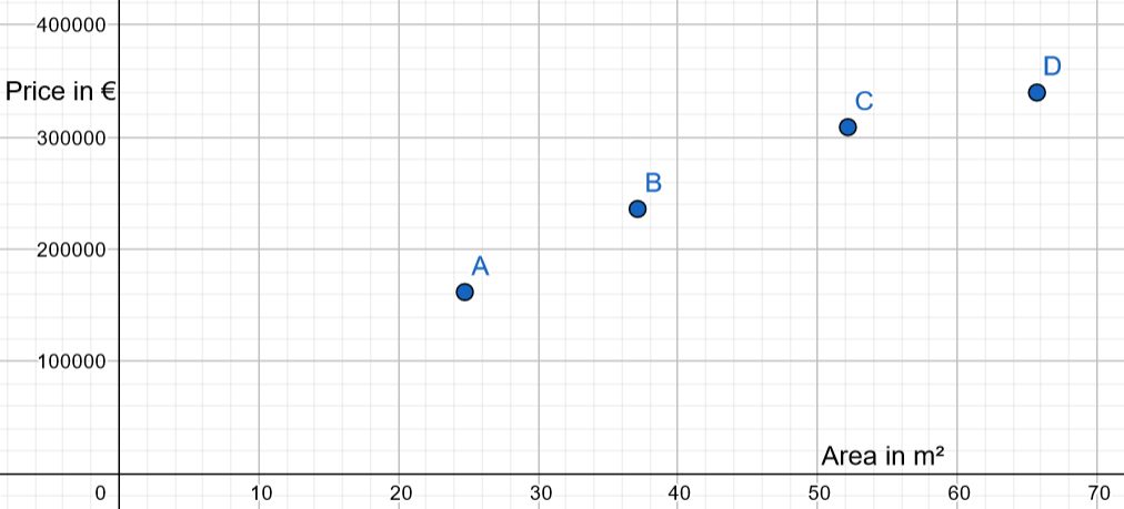
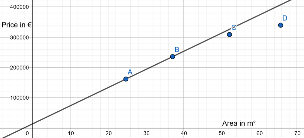
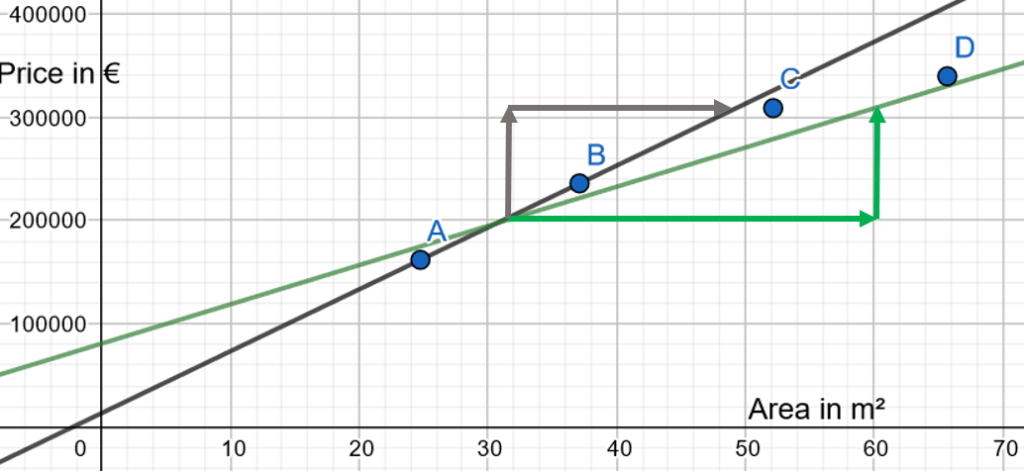
The graphical plot of your dataset is:

A first idea could be to draw a linear function:

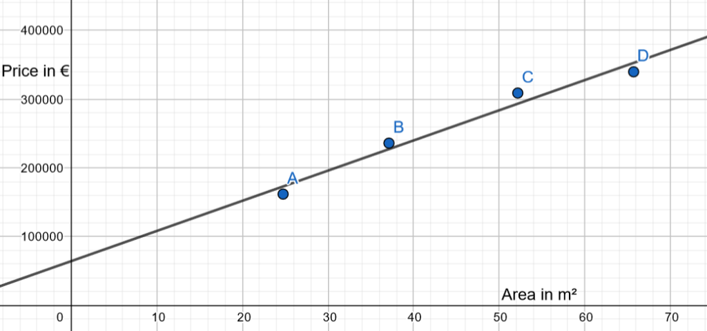
It would be interesting to arbitrarily split the dataset into:

Training data: for instance, A and B
Test data: for instance, C and D

And to create a linear function only with A and B and then measure the error with C and D:

Why is the dataset not exactly linear?

Indeed, in real estate, price is not a linear function depending on the area: see the average prices (Prix m² Moyen), in the 2010ies, in the 20th district of Paris, compared to the number of rooms (in France, adding living room + bedrooms provides the number of rooms):

prix m2 paris : calcul par appartement — Source: https://www.dimo-diagnostic.net

When the number of rooms increases, the € price per m² decreases.

Hence, we could consider a different slope, which means we could use a different linear regression coefficient.

A dataset example based on the previous table:

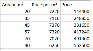
Some examples from the previous diagram with arbitrary areas but the realistic corresponding number of rooms in Paris

Plotting this example:

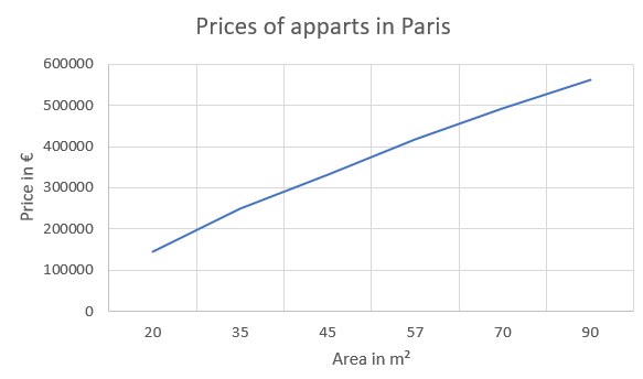
**The slope has less weight when the area is increasing**

So we will try to consider the degressive price per m² in this real estate dataset example.

A reminder of the classical metric of linear regression: the mean squared error

Sorry, we need to go abstract as little as possible.

Linear regression provides an analytical solution when minimizing the mean squared distances: Linear regression

In this clumsy proposition of linear regression:

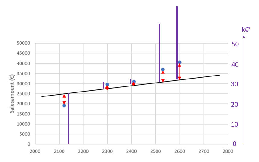
Firstly, we measure the distance between all the points and the proposed line:

Secondly, we square all these distances:
Remark: in order to improve understanding, we are counting in thousands of €, called k€.

The first point’s distance is 25-20 = 5 k€.

When we square it, it becomes 5*5 = 25 [k€]².

The square distances are roughly plotted in violet. As the squared distance is €² and not €, we need a new scale at the right of the plot.

Thirdly, we sum all these squared distances:

The sum is around 90 [k€]²

Fourthly, we need to calculate the mean.

The sum squared distance is 90 [k€]², and we divide it by the number of points, that is 5.
The Mean Square Distance, or Mean Square Error is roughly 90 / 5 = 18 [k€]².

Introduction of the Ridge and Lasso concept

With this micro dataset example of 4 observations, we have arbitrarily split it into 2 datasets of 2 observations, train A&B, and test C&D.

We have noted the slope, despite being analytically correct, might be improved with a lower weight.

The average price per m² of apartments decreases a little with high m² values:

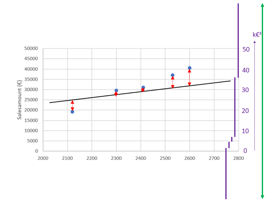
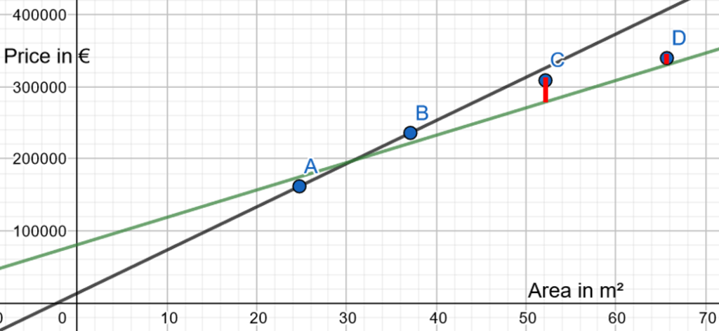
In our arbitrary example, if we only consider the first two observations of Train A&B, the slope would be in orange:

And we will schematically illustrate how Lasso and Ridge could adapt this into a slope in green:

In other words, we would like to diminish the weight of the single explanatory variable, with a mitigation of the slope.

This is the aim of Lasso and Ridge.

Conclusion of the concept with one-variable example

In this first part, we have introduced a Real Estate apartment example, with the area as the variable.

The linear regression doesn’t provide the best parameters of intercept and slope when knowing the price of apart is not precisely linear when the area is increasing.

We will adapt the metric Mean Square (MSE) described in this post by adding a curious penalty, involving a parameter called Lambda λ. We will try to find the best value for this new parameter λ.

Application of 1-variable example

Disclaimer:

With only one variable, Lasso and Ridge are globally useless, as basically the aim is to determine the most relevant variable(s).

Hence, the aim of this post with one variable is only to provide an understandable and visual example.

So, we will see in a future post, an example with two variables.

In the first post, we collected a dataset of fourth observations.

We have determined that two observations (A and B) will be used as training data and the last two observations (C and D) as test data.

With the test data (A and B) we have drawn a linear regression dataset function with the test function:

Now we will study the result with the test data (C and D).

Analysis of test data (C and D)

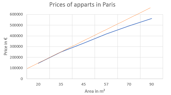
The linear applied with test data is not awful:

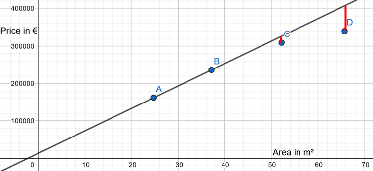
Nevertheless, there is a classical phenomenon in Data Science: the linear regression is perfect with our training data, but not perfect in our test data, as there is there an overfit.

If we draw the linear regression only with test data, the result is:

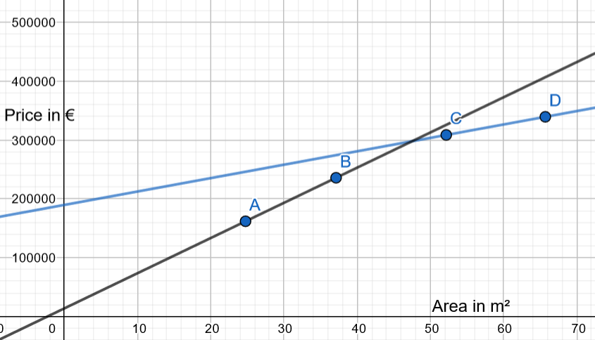
We still want to define a linear regression based on our test data, but we also are looking for a way to improve it.

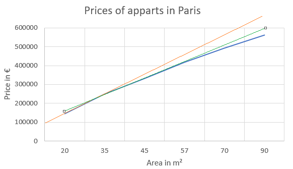
Ideally, we need to find a new green line, determined from testing data, with a lower slope, that would reduce the error, thus acknowledging that the price per m² is decreasing when the m² are increasing:

What is the meaning of a lower slope?

For the same increase of flat price, our target blue line needs a bigger increase of area:

In other words, our target is to reduce the weight of the variable « Area ».

The lambda parameter: λ

We define an improved linear regression.

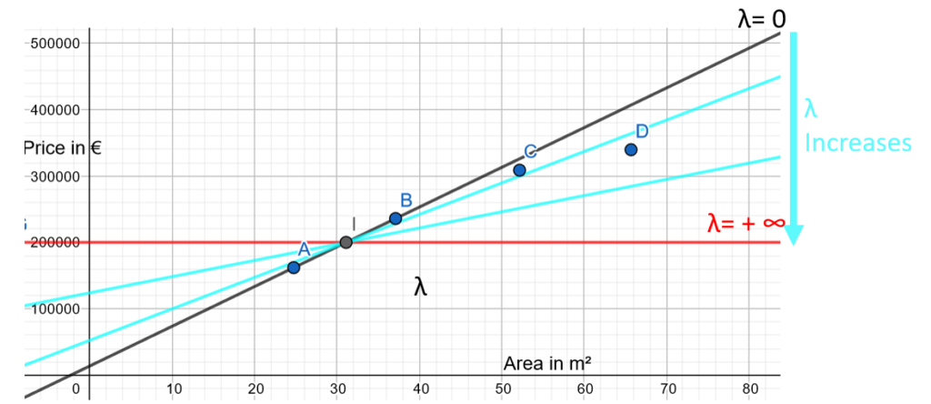
We define a parameter, with a value between 0 and +∞, which we call the lambda parameter λ.

The classical linear regression aims to minimize the metric called Mean Square Error.

We add a penalty to the Mean Square Error metric:

For Ridge, the penalty is Lambda multiplied by the square of the slope.
- The new metric is Mean Square Error + λ * (linear regression slope)²
For Lasso, the penalty is Lambda multiplied by the absolute value of the slope.
- The new metric is Mean Square Error + λ * |linear regression slope|

The way with one single value of lambda:

You arbitrarily decide on the value of λ
You run a Ridge/Lasso Regression, which uses different calculations than Linear regression, as the metric is different
The Ridge/Lasso regression will provide a new coefficient
- If λ is close to 0, then the metric Mean Square Error + λ * (linear regression slope)² is close to the Mean Square Error. Hence, the result will be close to the initial linear regression.
- If λ is converging to +∞, then the metric Mean Square Error + λ * (linear regression slope)² is converging to λ * (linear regression slope)². It must be reminded that the penalty has been chosen such that it reduces the weight of the variable. With λ converging to +∞, the weight converges to 0, then the slope converges to 0: in other words, when lambda is close to +∞, then the line is close to a horizontal line.
- With λ with a range of values from 0 to +∞, then the result is a set of lines in a range from the initial slope to a horizontal line.

Two examples with different lambda values

Finding the right λ value

Manually & basically, the job would be to :

Define a range of multiple values between 0 to +∞.
With the train data, determine the slope for each λ value.
With the test data, calculate the error for each λ value.
To compare all the errors, and to pick the λ value with the minimal error.

Happily, there are functions, at least with R languages, that do all these steps and provide the optimal lambda value.

It’s time to apply our example with R programming.

Application of Ridge/Lasso with R programming

Just a reminder and disclaimer: Lasso and Ridge are non-sense with only one explanatory variable. As we needed an understandable graphical example plotted in 2D with one explanatory variable, we are twisting the library for this 1-variable real estate example: we will add a dummy column with only a « 0 » value for each observation so that the function will consider this example as 2-variable.

First, we call our libraries.

```{r}
# We call the data.table library
library(data.table)
# glmnet is the classical R library for Lasso and Ridge
library(glmnet)
```

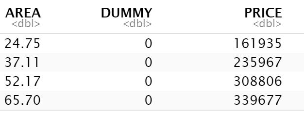
Then we create our dataset as data.table.

```{r}
# "DUMMY" dummy variable added, as the function 
# is required at least 2 columns of variables
dt_apart <- data.table(
            AREA =  c(24.75,  37.11,  52.17,  65.70),
            DUMMY = c(0,      0,      0,      0    ),
            PRICE = c(161935, 235967, 308806, 339677)
)
head(dt_apart)
```

We prepare an input matrix with PRICE and DUMMY, and an output vector with PRICE.

```{r}
# input variables AREA and DUMMY
x <- data.matrix(dt_apart[, -3]) # -3: we remove the third column
# output variable
y <- dt_apart$PRICE
```

We run a Lasso model with our dataand use cross-validation. In summary, instead of using only A and B as training data and only C and D as test data, we work with all possible 2-observation test data and all possible 2-observation training to avoid overfitting.

https://en.wikipedia.org/wiki/Cross-validation_(statistics)

# alpha = 1 -> Lasso penalty
# alpha = 0 -> Ridge penalty

# We decide to run the model with Lasso
apart_model <- cv.glmnet(x, y, alpha = 1)

# We just need to ask to glmnet what was the optimal lambda
optimal_lambda <- apart_model$lambda.min
View(optimal_lambda)

The optimal lambda value is 1972.01
Also, you can see that *glmnet* has noted we have used a dataset with very little data

We are plotting the model.

```{r}
plot(apart_model) 
```

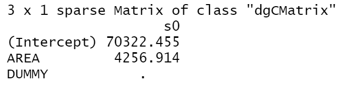
It is not graphically obvious that the minimum is at Log(1972.01) = 7.59. Happily, a vertical dotted line is notifying it.

Now we call the intercept and slope (coefficient) of the Lasso model:

**Interpretation: For each new m², the price of the flat is increasing by 4256 € with our Lasso model**

We want to compare with linear regression.

Reminder: with the linear regression, lambda = 0

```{r}
# with lambda = 0, it means it is linear regression
lr_apart_model <- glmnet(x, y, alpha = 1, lambda = 0)
coef(lr_apart_model)
```

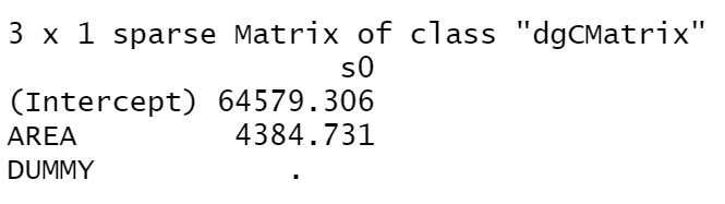
For each new m², the price of the flat is increasing by 4384€ with our Lasso model

As a summary, the comparison with Lasso and Linear regression:

Variable	Initial Linear model	Our Lasso model
Intercept Theoretical price of a flat when the area is 0 m² Remark: compared to reality, it means the less area, the less precision of the linear model	64580	70320
Slope coefficient for each new m², the price of the flat is increasing by	4384	4256

In a conclusion, following our twisted methodology, we have managed with Lasso to withdraw the weight of the area in m² of the flat.

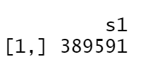
If our prospect flat has an area of 75 m², what is the predicted price?

```{r}
# Define an flat of 75 m²
new_apart <- matrix( c(75, 0), nrow = 1, ncol=2)
# Ask the prediction with the Lasso model
predict(lasso_apart_model, s = optimal_lambda, newx = new_apart)
```

With the Lasso model, the predicted price is almost 390.000 €

# Ask the prediction with the Linear regression model
predict(lr_apart_model, s = 0, newx = new_apart)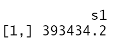

With the Lasso model, the predicted price is around 393.000 €

Conclusion of the one-variable example

We had initially decided to work with a linear model, a model with one explanatory variable.

For didactic purposes, we wanted to consider the following real estate rule: the price of a flat is not a linear function: when the number of rooms increases and the area increases, then the € price per m² decreases.

Also, we knew, as a business rule, that the flat to predict had a greater area.

So we have « curved » the linear model and have created a lambda parameter that has reduced the weight of the price per m².

With a flat of 75 m², we have managed to reduce the prediction of the flat price of 3000€ from the linear model, which is business-wise.

A reminder: don’t use Lasso or Ridge with only one explanatory variable: this example was a learning curve ramp-up to introduce the lambda parameter.

Lasso and Ridge Regression