Isotonic Regression

Introduction to the problematic

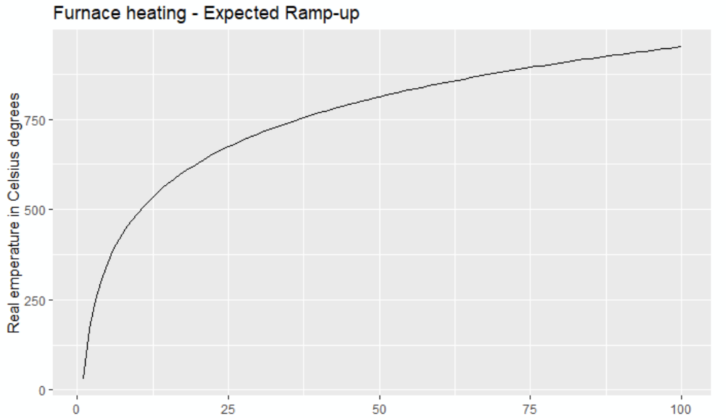
Imagine a research lab testing a furnace requiring no progressive heating and no threshold.7

The expected temperature ramp-up should look like this:

Unhappily, there is only one sensor, and it is faulty: the measured result is like hereunder:

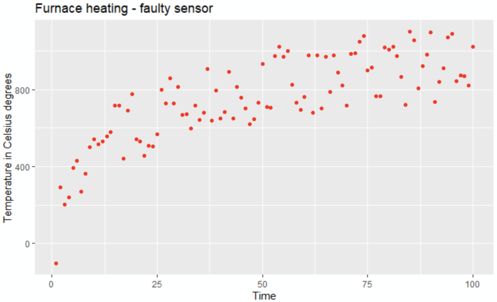
The sensor indeed seems to have a gaussian error

How could we estimate the temperatures, from these observation temperatures?

The definition of isotonic

The isotonic or monotonic regression applies when a function is non-decreasing all the time, or non-increasing all the time

A monotonic non-decreasing function:

A monotonic non-increasing function:

A non-monotonic function:

What does an isotonic regression look like?

It is a regression, non-decreasing or non-increasing, which fits the observations.

Hereunder, the red line is a non-decreasing regression:

How is calculated the isotonic regression?

The algorithm is very mathematical, too much for vulgarization; hence we’ll approach superficially the isotonic regression definition:

like the linear regression, the aim is to find some points with the least square method https://en.wikipedia.org/wiki/Least_squares
with the additional constraint of increasing or stable points in case of a non-decreasing function, or decreasing or stable points in case of non-increasing function, instead of linear definition

You can find some explanation at this link:

R programming: catch-up of the introduction example

Here you are the R language code which has provided the introduction data and plots from the introduction of this post.

The package declaration:

# Declaration of package for high-level plotting
library(ggplot2)

The generation of the furnace data:

# As the runif function will generate random numbers, we want to reproduce the data
set.seed(3)
# We create 100 time points
i <- 100
x <- seq(1,i)
# We create the real temperature timeline of the furnace with a logarithmic function
y <- 30 + 200 * log(x)
# We simulate faulty sensors, with gaussian error, between -200°C and +200°+C
error <- runif(100, -200, +200)
# The data is stored as data.frame. data.table often is not recognized with the future packages
df_furnace <- data.frame( TIME = x, REAL = y, SENSOR = y + error)
head(df_furnace)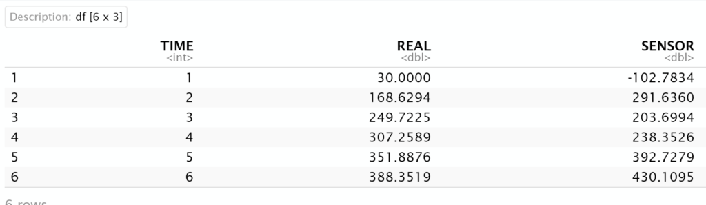

The REAL data plot:

# Plotting the real data
ggplot(df_furnace, aes(TIME, REAL) ) + geom_line(color = "black") + labs(title = "Furnace heating - Real temperatures") + xlab("Time") + ylab("Real emperature in Celsius degrees")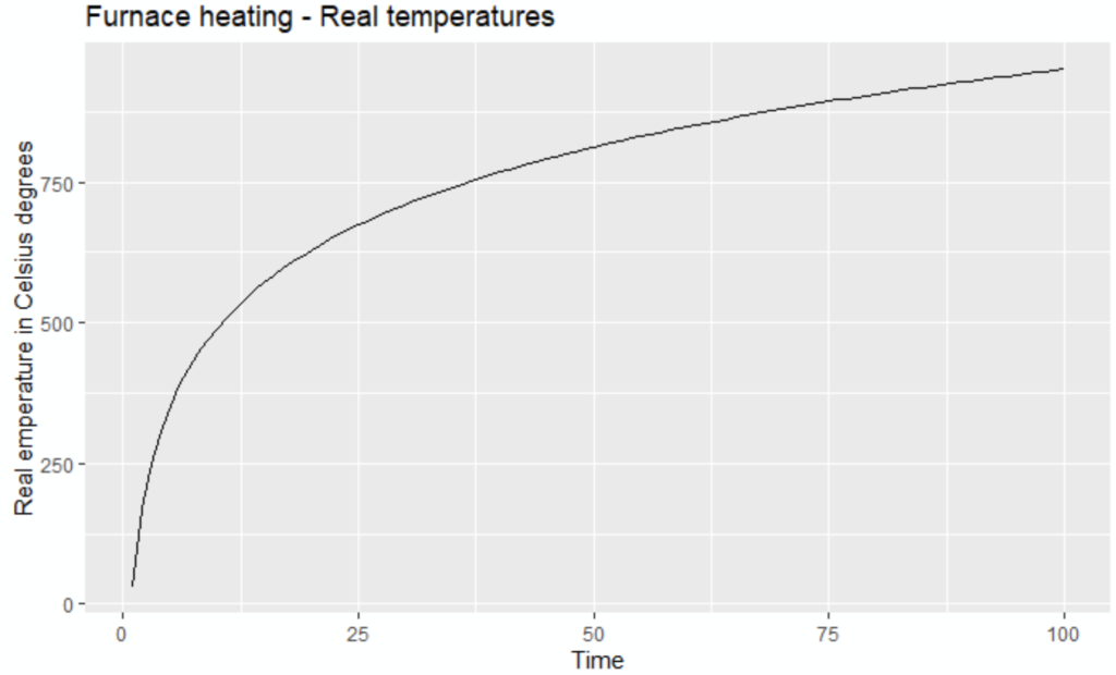

The SENSOR data plot:

# Plotting the sensor data
ggplot(df_furnace, aes(TIME, SENSOR) ) + geom_point(color = "red") + labs(title = "Furnace heating - faulty sensor") + xlab("Time") + ylab("Sensor temperature in Celsius degrees")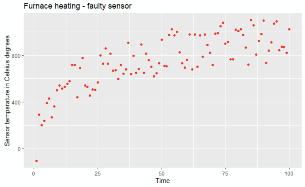

R programming: linear regression as reference

This paragraph aims to remind us of linear regression before comparing it to isotopic regression in the next paragraph.

# Calculation of the linear regression model
lr_model <- lm(SENSOR ~ TIME, data = df_furnace )

# Extract the fitted value calculated by the linear model
df_furnace$LINREG <- as.data.frame(fitted(lr_model))[,1]

# Plot the linear regression
ggplot( df_furnace, aes(TIME,SENSOR)) + geom_point( aes (y = SENSOR, colour = "Sensor") ) + geom_line( aes (y = LINREG, colour = "Linear Regression") ) + geom_line( aes (y = REAL, colour = "Real") ) + labs(title = "Linear regression") + scale_colour_manual("",  breaks = c("Sensor", "Linear Regression", "Real"), values = c("red", "green", "black")) + ylab("Temperature °C") + xlab("Time")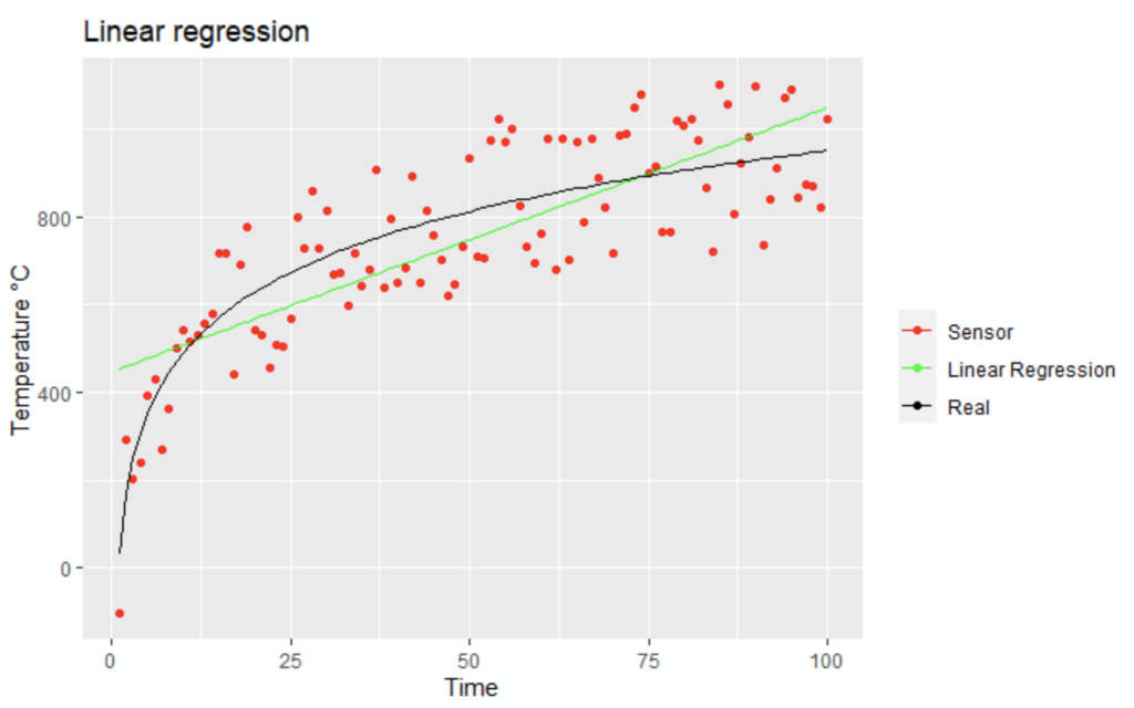

R programming: isotonic regression example with Iso library

# We have arbitrarily chosen the "iso" package
# https://cran.r-project.org/web/packages/Iso/Iso.pdf
library(Iso)

We calculate the isotopic regression model:

# Calculate the Isotopic Regression model
ir_model <- isoreg(df_furnace$TIME, df_furnace$SENSOR)
df_furnace$ISOREG <- ir_model$yf
# Display the first isotonic regression temperatures
head(df_furnace$ISOREG)

Now we plot the result:

# Plot the isotopic regression
ggplot( df_furnace, aes(TIME,SENSOR)) + geom_point( aes (y = SENSOR, colour = "Sensor") ) + geom_line( aes (y = ISOREG, colour = "Isotonic Regression") ) + geom_line( aes (y = REAL, colour = "Real") ) + labs(title = "Isotonic regression with Iso package") + scale_colour_manual("",  breaks = c("Sensor", "Isotonic Regression", "Real"), values = c("red", "blue", "black")) + ylab("Temperature °C") + xlab("Time")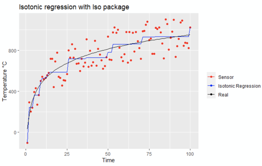

Here the isotonic regression has a typical « stairway » shape

The Isotonic regression smoothing seems to fit better, let’s confirm graphically:

# Compare the linear regression VS the isotonic regression
ggplot( df_furnace, aes(TIME,REAL)) + geom_line( aes (y = ISOREG, colour = "Isotonic") ) + geom_line( aes (y = LINREG, colour = "Linear") ) + geom_line( aes (y = REAL, colour = "Real") ) + labs(title = "Linear regression VS Isotonic regression") + scale_colour_manual("",  breaks = c("Isotonic", "Linear", "Real"), values = c("blue", "green", "black")) + ylab("Temperature °C") + xlab("Time")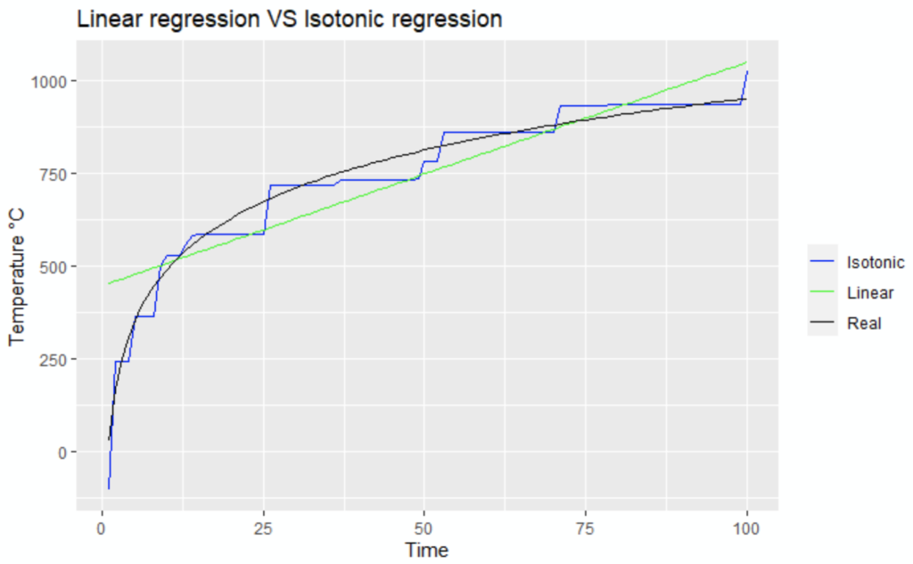

The blue line / isotonic regression is definitely closer to the black line / real data than the green line / linear regression!

Conclusion

When a function has a non-decreasing or non-increasing property, this constraint helps to smooth fitting with proper tools.

We have applied an example of isotonic regression, which is the basic tool for this kind of constraint.

There are other tools that provide better results for smoothing or prediction: we will study them in an upcoming post