Theory
Introduction
Data cleaning is crucial in Data Science.
The data usually are dirty when the Data specialist is required because:
- If the data were clean, it would surely be easier to understand, and somebody would already have extracted intelligence without the data scientist.
- Life is noisy in many domains, like Economy, Industry, Science, and Medicine. For example:
- Human behavior can differ between groups of people. Even for one single human, behavior can change according to timelines, circumstances, cues, or even be random.
- An outcome often is the result of many parallel and/or serial steps, which have slight differences at each occurrence: the same vineyard will provide each year a different wine taste because of varying hygrometry, temperature, sunshine, rain, nutrient supply, vinification: https://vgir.fr/2021/03/16/the-normal-distribution-why-is-it-recurring-in-nature/
Comprehension is the key to data cleaning
Unhappily there is no guide or recipe for data cleaning. Only some very general rules can be provided.
There are three rules as important as difficult to define:
- 1 – The data must be understood from a business point of view.
- 2 – The data tools and algorithms must also be understood, in order to anticipate the data-cleaning impacts.
- 3 – Guess-and-check methodology.
1 – The data must be understood from a business point of view
For example, you could find a correlation between the total per capita consumption of chicken and the Total US crude oil imports; see hereunder plot:
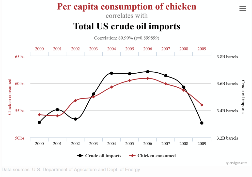
By getting more information from the US Department of Agriculture and the US Department of Energy, could one or both the correlated data time series be cleaned and get a better correlation? Or a causal link?
Indeed, the data are only correlated without a causal link, meaning they randomly occurred. Save time: there is no cause-and-effect relationship.
https://en.wikipedia.org/wiki/Correlation_does_not_imply_causation
The cleaning methodology and options must be adapted to each dataset based on business comprehension.
2 – The data tools and algorithms must also be understood
For example, if you have a dataset of 100 humans, with one column being the age, this age column is not filled out for 90 observations. All other columns are fully filled. What should you do?
Some possibilities:
- Remove the entire column?
- Keep the column as is with some missing values?
- Try to guess the age from other columns?
Example: trying to guess the age from the first name
- The underunder examples applies only for France
- If the first name is Mickael, an active worker is not an unreasonable guess, so why not indicate 45 as the age?
- If the first name is Jean, a retiree is not an unreasonable guess, so why not indicate 70 as the age?
- If the first name is Ambre, a child or young adult is not an unreasonable guess, so why not indicate 20 as the age?
- Bad luck, some first names have no temporality like Sophie
- A reasonable guess is far from certainty, so why not set the mean age of the dataset observations whose age is known? Why not set the mean age of the population to which the dataset belongs, like its country?
Some business questions are raised, still with this missing age example:
- What happens if the guess age is totally wrong? Does it depend on the algorithm later used? It is better to remove the entire column?
- How reliable is the model if only ten observations are kept?
- Indeed, is age important? Could the column be removed?
Some examples detailing why the technical understanding is important:
- If we try to appy a linear regression, the values cannot be empty. And sacrifying 90% of the observations is risky.
- If we try to apply a decision tree, the missing values are not an issue.
3 – The guess-and-check methodology
It’s normal not to be sure about the consequences of all the possible data cleaning methods.
Finally, it’s a good idea to guess and check: the guessing part will save time by removing the obviously non-sense options. The result should provide useful output.
The checking partis a comparison to validate the guesses. And if you have time, you can always check later the nonsensical options: yes, even when understanding the business, some counterintuitive facts can be discovered.
With the missing age example, it is advised to check, indeed to compare, to evaluate some already guessed options…
Compare many ways such as:
- The decision tree with the age column.
- The decision tree without the age colum.
- The linear regression without the age column.
- The linear regression with only the age column filled, meaning only ten entries are kept.
- The linear regression with the age column corrected, meaning with all 100 entries
- with the different methods:
- age mean.
- age guessing.
- …
- with the different methods:
The comparisons will help determine which are the best, or at least which seems the least bad choices.
Common cleaning steps
Remove wrong observations or data
The idea is to remove the observations or at least deal with the incorrect data.
A colleague dealing with HR data in a big French energy company extracted the entire dataset of active employees.
A couple of active employees were 100+ years old : it was obviously a mistake.
The options:
- Check if the employee is still active. If not, the retirement switch may have been forgotten, and the observation should be removed from the dataset.
- Asking the business to correct the date of birth information.
- If you can’t get quick help, remove the dataset, as the aim is an economic study, and removing several observations on a dataset with 100,000+ observations is not an issue.
Remove unneeded columns
When you receive files with many columns, you may already know, from a business point of view, that some columns are irrelevant.
The models will run faster. And sometimes, it is even mandatory to get a lighter dataset. For instance, if you have received a huge dataset but have limited computer memory or calculation power.
Remove duplicates
It happens to find duplicates, either there was a business error (filling twice the data), or a technical error (mistake with data aggregation)
Structural errors
It could be summarized as typos, some examples:
- Union of two files, the years 2020 and 2021, one has a column Create_Date and the other Creation_date: despite the column names are different, they have the same meaning and should be merged.
- Some columns could have different empty indicators, such as NaN, N/A, or Not Applicable, which need to be uniformized before further processing.
- Date formats could be mixed, like 31/01/2021, 01/31/2021, 01.01.2021.
- Classification could be mistaken: blu entered instead of blue.
Remove or manage outliers
An outlier can be unrealistic, as the centennial active workers mentioned above. But it could also be a value that is too great or too low compared to the usual values.
For example, a sensor usually indicates a furnace between 1000 and 1100 degrees Celsius. If there is a single value of 1800 °C, indeed this is an error from the sensor: the observation could be removed: https://vgir.fr/isotonic-regression/
Deal with missing data
This has already been developed with the age example. Let’s summarize the options:
- Drop the observation
- Imput the missing value: it means to find a susbtitute value.
- In the best scenario, replace the missing value with a most approaching value: for example, guessing the age, fetching a mean or median value.
- In worst scenario, for a missing numeric value, an arbitrary value, could also being set, if it is not possible to do better: for example 20 for the age, if the dataset concerns only students, as 20 is the median of the dataset.
- For a missing category like the color blue, green, or red, a missing category like the color unknown could be created.
- Finding a tool to deal with the missing value: As mentioned before, decision trees can work without the value, in contrast to linear regression.
Evaluate qualititively the previous steps
In each previous step, you have tried to apply the best solution, based on your data and business knowledge, and on your experience.
It is important to check:
- After cleaning, do the data still seem good for an analysis?
- Does the analysis result is consistent?
- Is the cleaning enough? Should it be improved? For the following analysis, less cleaning could gain time without degrading the result?
- Does it validate or not the expected theory or model? Why?
- If you find no conclusion, it is still a cleaning issue? Maybe even spending several years in cleaning, nothing can be extracted from the data? Maybe the data are beyond cleaning?
- For example, if you try to predict the NASDAQ, whether the data is clean or not, failing is almost a guarantee.
- For exemple, if a faulty and essential sensor is providing such wrong measures, just stop the analysis, ask its replacement, and then start again the data analysis.
As a reminder, the quantitative evaluation has already been mentioned in the Guess-and-check part
Conclusion of the data cleaning’s theory
It’s unhappily usual to receive dirty data. In this case, cleaning is necessary, and it usually needs a huge amount of time.
There is no standard procedure to apply; only some best practices must be followed. Cleaning requires common sense, an understanding of the business, a consideration of the tools and algorithms that will use this data, and a try-and-guess to validate the hypothesis.
Sometimes the data are such dirty, that it is beyond cleaning: this possibility must always be remembered, in order to either mitigate the expectations or even cut the losses, like postponing the data science project when new correct data can be provided, or even stopping the project.
It’s essential to clean the data as soon as possible, even before the data science project; for example, repairing the sensors in a furnace, instead of dealing with erroneous data: https://vgir.fr/isotonic-regression/
In the next few pages, we’ll apply data cleaning to a 2021 real estate dataset from the French Val-de-Marne county, which will highlight the criticality of business comprehension.
Example: deeds of sale – part 1
First, we will extract the 2021 first semester of deeds of sale of apartments and houses for the Val-de-Marne department:

In France, the department is a subdivision similar to the county in the USA.
We will clean the data with R language:
- Delete the useless or almost useless columns to avoid overfitting.
- Clean the useful columns.
- Also, clean the observations. For instance, as we are interested only in houses and parts sales, we need to remove land, industrial properties, and other non-living estates.
The aim is to predict the prices of houses and apartments according to the explanatory variables in future posts, starting with algorithms based on decision trees.
The Val-de-Marne deeds of sale
These « open data » datasets Demande de valeurs foncières géolocalisées can be found at: https://www.data.gouv.fr/fr/datasets/demandes-de-valeurs-foncieres-geolocalisees/

The download part looks like this:
Click on the icon:

The result is:
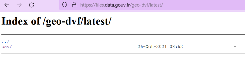
Click on csv/:
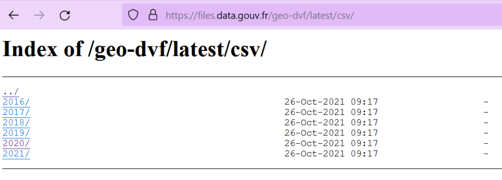
Select the latest year:
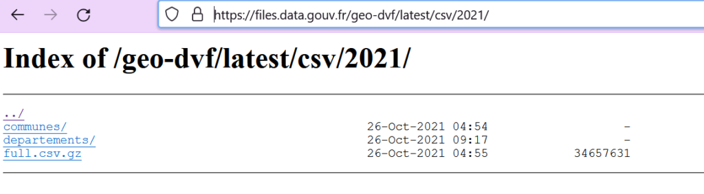
full.csv.gz would provide the data for mainland France, Corse, Guadeloupe, Martinique, and La Réunion islands.
To work with a lighter file, we have chosen to deal with only one department, the Val-de-Marne. Whatever the file, city, department, or full scope, the column structure will remain the same.
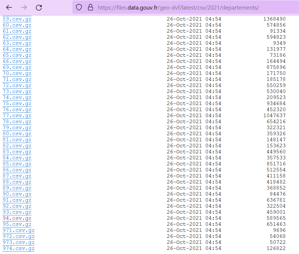
If the sub-directory departments/ is chosen:
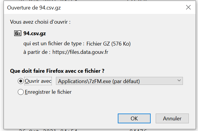
Save the file:
The file can be extracted with 7zip: https://www.7-zip.org/
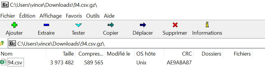
You get the file 94.csv:

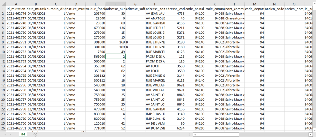
The columns of the file
They are described in french:
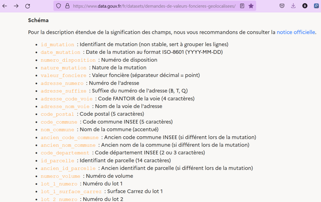
Let’s create our own English translation.
Do not focus on the business content, the columns will be later detailed, to justify the data cleaning, column after column:
| # | ID of column | FRENCH DESCRIPTION | ENGLISH DESCRIPTION |
| 1 | id_mutation | Identifiant de mutation (non stable, sert à grouper les lignes) | Deed ID (generated and also anonymous, we’ll detail why and how it is required) |
| 2 | date_mutation | Date de la mutation au format ISO-8601 (YYYY-MM-DD) | Deed date with format YYYY-MM-DD |
| 3 | numero_disposition | Numéro de disposition | An incremental sub-number for each id_mutation |
| 4 | nature_mutation | Nature de la mutation | Type of deed (Sales, expropriation…) |
| 5 | valeur_fonciere | Valeur foncière (séparateur décimal = point) | Sales amount: the field to be predicted. Value in EUR, the decimal separator is « . » |
| 6 | adresse_numero | Numéro de l’adresse | Street number |
| 7 | adresse_suffixe | Suffixe du numéro de l’adresse (B, T, Q) | Street number suffix (Bis, Ter, Quater) |
| 8 | adresse_code_voie | Code FANTOIR de la voie (4 caractères) | Type of street: street, avenue, boulevard… |
| 9 | adresse_nom_voie | Nom de la voie de l’adresse | Street name |
| 10 | code_postal | Code postal (5 caractères) | Postal code (5 digits) |
| 11 | code_commune | Code commune INSEE (5 caractères) | Alternative postal code, used by statistic institute |
| 12 | nom_commune | Nom de la commune (accentué) | City name |
| 13 | ancien_code_commune | Ancien code commune INSEE (si différent lors de la mutation) | Old city ID (for example in case of city grouping) |
| 14 | ancien_nom_commune | Ancien nom de la commune (si différent lors de la mutation) | Old city name (for example in case of city grouping) |
| 15 | code_departement | Code département INSEE (2 ou 3 caractères) | Department code |
| 16 | id_parcelle | Identifiant de parcelle (14 caractères) | Parcel ID |
| 17 | ancien_id_parcelle | Ancien identifiant de parcelle (si différent lors de la mutation) | Old parcel ID |
| 18 | numero_volume | Numéro de volume | Sub-increment |
| 19 | lot_1_numero | Numéro du lot 1 | ID of first batch |
| 20 | lot_1_surface_carrez | Surface Carrez du lot 1 | Living space of first batch in square meters |
| 21 | lot_2_numero | Numéro du lot 2 | ID of second batch |
| 22 | lot_2_surface_carrez | Surface Carrez du lot 2 | Living space of second batch in square meters |
| 23 | lot_3_numero | Numéro du lot 3 | ID of third batch |
| 24 | lot_3_surface_carrez | Surface Carrez du lot 3 | Living space of third batch in square meters |
| 25 | lot_4_numero | Numéro du lot 4 | ID of fourth batch |
| 26 | lot_4_surface_carrez | Surface Carrez du lot 4 | Living space of fourth batch in square meters |
| 27 | lot_5_numero | Numéro du lot 5 | ID of fifth batch |
| 28 | lot_5_surface_carrez | Surface Carrez du lot 5 | Living space of fifth batch in square meters |
| 29 | nombre_lots | Nombre de lots | Number of batches |
| 30 | code_type_local | Code de type de local | Type of estate ID: aparment, house, land… |
| 31 | type_local | Libellé du type de local | Type of estate description: aparment, house, land… |
| 32 | surface_reelle_bati | Surface réelle du bâti | Real built area in square meters |
| 33 | nombre_pieces_principales | Nombre de pièces principales | Counting every room, also including living room… |
| 34 | code_nature_culture | Code de nature de culture | Code of culture: land, water, forest… |
| 35 | nature_culture | Libellé de nature de culture | Type of culture: land, water, forest… |
| 36 | code_nature_culture_speciale | Code de nature de culture spéciale | Code of special culture: pond, wasteland, vegetable garden… |
| 37 | nature_culture_speciale | Libellé de nature de culture spéciale | Type of special culture: pond, wasteland, vegetable garden… |
| 38 | surface_terrain | Surface du terrain | Land area in square meters |
| 39 | longitude | Longitude du centre de la parcelle concernée (WGS-84) | Longitude |
| 40 | latitude | Latitude du centre de la parcelle concernée (WGS-84) | Latitude |
Opening the file with R language
We use data.table library for its efficiency:
```{r}
library(data.table)
```
We read the Demande de valeurs foncières dataset.
The encoding = ‘UTF-8’ is required or there will be an issue with french accents:
```{r}
vf <- fread("C:\\Users\\vince\\...\\94.csv", encoding = 'UTF-8')
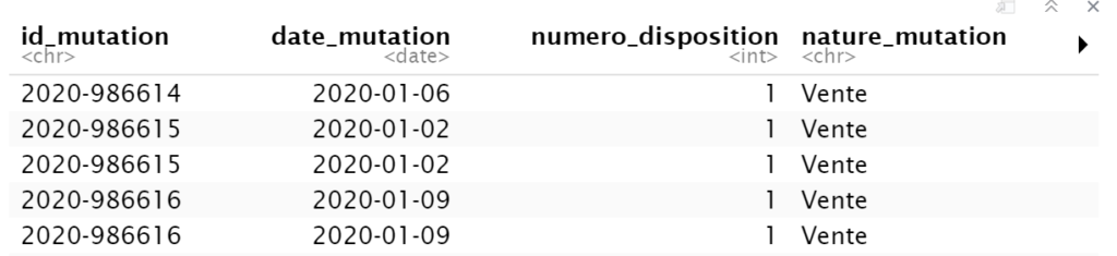
head(vf)
```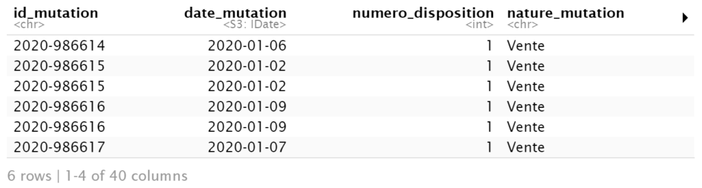
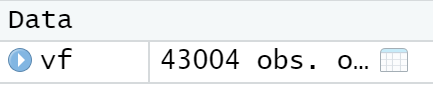
It also looks like this in the R studio environment:
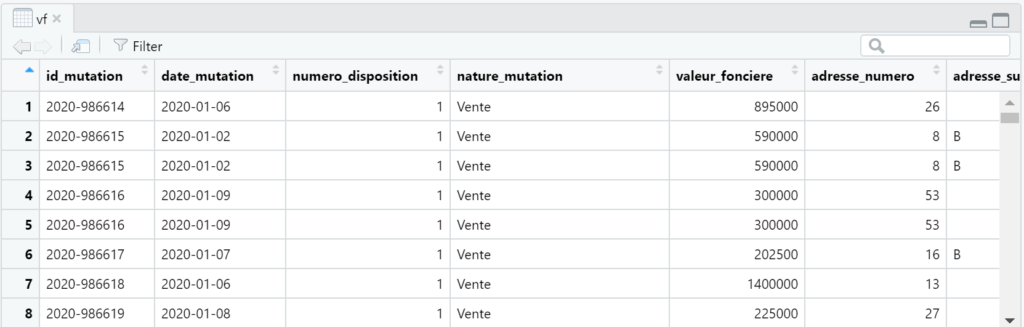
There are 43004 rows, so it won’t have high memory requirement:
Conclusion of the example – part 1
We have learned to download the sales deeds file for the county of Val de Marne.
It contains 40 fields: some of them are useless, some of them need to be reworked, and we’ll discover that some lines need to be grouped in the next posts, with R programming.
Example: deeds of sale – part 2
Data cleaning of columns
1- id_mutation column
French: Identifiant de mutation: non stable, sert à grouper les lignes.
English: Deed ID: generated and also anonymous, we’ll detail why and how it is required.
This is a generated ID providing anonymity, and its aim is to group the rows: its usefulness will be explained in a future post.
```{r}
### We keep it as-is the time being
```
2- date_mutation column
French: Date de la mutation au format ISO-8601 (YYYY-MM-DD)
English: Deed date with format YYYY-MM-DD
The date is kept if in the future we would like to study the evolution of real estate prices. With a dataset of 6 months, this is probably not significant, but with one or several years, it would become interesting.
We ensure this column is converted in a date format recognized by R language.
```{r}
vf <- vf[, date_mutation:= as.Date(date_mutation) ]
head(vf)
```
3- numero_disposition column
French: Numéro de disposition
English: An incremental sub-number for each id_mutation
```{r}
table(vf[ , numero_disposition])
```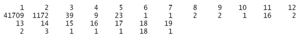
The value 1 -> 41709 times, the value 2 -> 1172 times…
This sub-counter doesn’t seem useful, as it is not a real increment: for instance, there are 9 entries of value 4 versus 23 entries of value 5.
We remove it.
```{r}
vf <- vf[, numero_disposition:= NULL ]
```
4- nature_mutation column
French: Nature de la mutation
English: Type of deed
We ask the possible values:
```{r}
print( unique(vf$nature_mutation))
```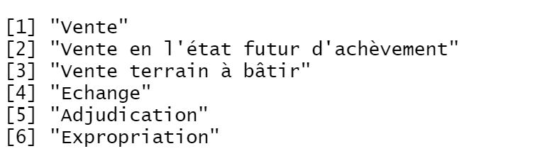
The possible values are
| French | English |
| Vente | Sale |
| Vente en l’état futur d’achèvement | Sale of estate not yet constructed: usually apartment |
| Vente terrain à bâtir | Land to build |
| Adjudication | Auction |
| Echange | Exchange |
| Expropriation | Expropriation |
We keep it, as, for example:
- Sale of estate not yet constructed usually allows to recognize new apartments buildings.
- Exchange may not indicate real market price
- Expropriation does not reflect consented sale of the market
- …
```{r}
# we keep it
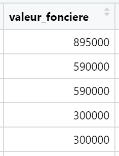
```5- valeur_fonciere column
French: Valeur foncière
English: Value of the estate
This is the value, in Euro currency, with . as decimal separator
This is the value of apartments or houses we will try to predict in several posts in the future, like with decision tree algorithms: mandatory, we keep it.
```{r}
head(vf[, c("valeur_fonciere")])
# we keep it
```
6- adresse_numero column
French: Numéro de l’adresse
English: Street number
In France, the prices of real estate usually are at first sight homogeneous across the same street in villages and small cities, and regularly in medium and big cities due to the reasons considered globally:
- The streets are not long in France
- The street name could be globally prestigious like the Street Rue de Rivoli in Paris, or with bad reputation, but it hardly applies to somes numbers, or segment of streets
- The closer the street is to the center, the more exceptions: some street segments can be more strategic thanothers.
Remark: When linked with street name and city, the address number can influence the prediction. But as classical prediction algorithms consider variables to be independent, this information isn’t taken into account.
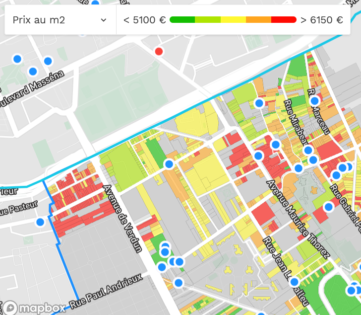
For example, hereunder, you can see that the prices are heterogeneous across the street numbers of rue Mirabeau in Ivry-sur-Seine. But the rule applies only to rue Mirabeau in Ivry. The distribution is different from the street numbers of rue Mirabeau in other cities, like Paris. Hereunder is also the screenshot ofrue Mirabeau in Paris.
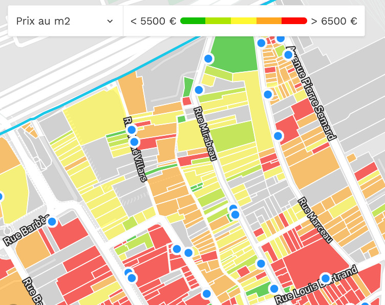
In conclusion, as an independent variable, the street number is not a good indicator of real estate prices, so we don’t keep this column [*]
6-  adresse_numero column
```{r}
vf <- vf[, adresse_numero:= NULL ]
```
7 – adresse_suffixe column
French: suffixe du numéro de rue: bis, ter, quarter… https://www.culture-generale.fr/histoire/87-origine-des-bis-ter-quater-dans-les-numeros-de-rue
English: suffix of the street number: bis, ter, quarter… http://www.aussieinfrance.com/2015/11/fridays-french-bis-ter-and-encore/
The suffix is like the sub-division of a street number. As street numbers are considered without influence, suffixes have even less influence: the column is not kept.
7- adresse_suffixe
```{r}
vf <- vf[, adresse_suffixe:= NULL ]
```
8 – adresse_nom_voie column
French: Nom de la voie de l’adresse
English: Street name
In France, all other things being equal, the city provides a very good first indicator of the value of an apart/house.
Then the district, if relevant, is a precise sub-indicator. Only the biggest french cities have districts: it is included in the postal code. For example, Paris has the department code 75, owns 20 districts, recognized by postal codes from 75001 to 75020.
For medium cities, a map is needed to recognize the administrative districts. Caution: There is no clear rule defining the districts. Also, districts can contain sub-districts with economically high amplitude.
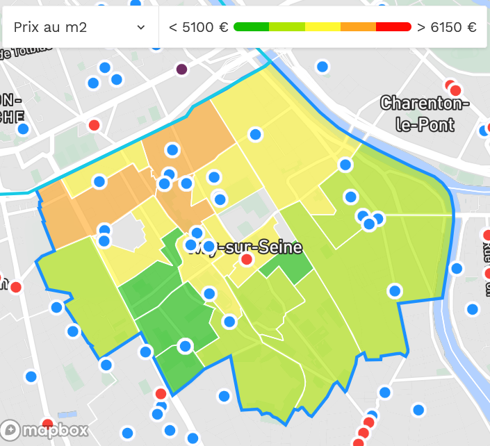
For example, the city Ivry-sur-Seine is divided into 6 districts:
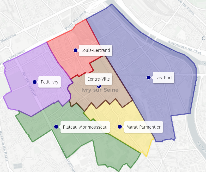
The districts have heterogeneous real estate prices:
Finally, focusing on street level:
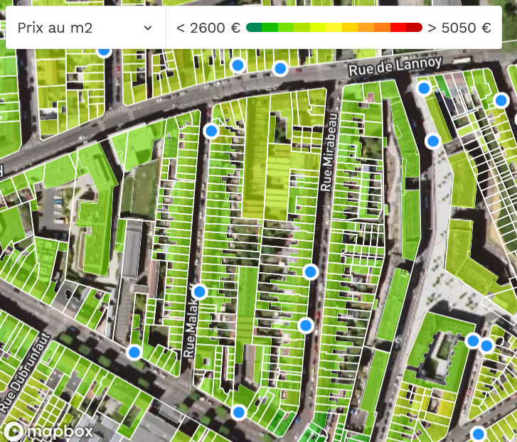
- Rue Mirabeau in Ivry-sur-Seine is in both popular, middle-class, and upper-class areas.
- Rue Mirabeau in Lille is in a more popular area.
- This comparison illustrates that the street name is not a good indicator of pricing when used as an independent variable.
In conclusion:
- The street name is an fair indicator of the real estate value, but only when coupled with the city.
- For example, rue Anatole France could be in a popular district in a city, and in a upper class in other city.
- As mentioned for the street names, classical prediction algorithms consider variables independent, so the street name in this context is not useful. [*]
We don’t keep the street name.
8 - adresse_nom_voie
```{r}
vf <- vf[, adresse_nom_voie := NULL ]
```
9 – adresse_code_voie column
French: Code FANTOIR de la voie (4 caractères) https://www.data.gouv.fr/fr/datasets/fichier-fantoir-des-voies-et-lieux-dits/
English: this is an administrative code for the street name.
We don’t keep the column, as we didn’t retain the column street name
```{r}
vf <- vf[, adresse_code_voie:= NULL ]
```
[*] Remark about dependant variables.
We have previously stated that street names and street numbers are bad indicators when considered as independent variables.
But the couple [street name, city] and the triple [street number, street name, city] accurately estimate pricing:
So their property could be used:
- In a prediction algorithm that can take into account the dependencies
- New variables could be created like:
- The concatenation of street name and city
- The concatenation of street name and street number and city
Conclusion of the example part 2
We have cleaned the 9 first columns of our real estate value file: we are resuming in a future post.
Example: deeds of sales – part 3
Data cleaning of columns
We resume at the tenth column.
10 – code postal column
French: code postal.
English: postal code / ZIP code.
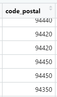
The postal code is a numerical identifier for cities: for instance, Ivry-Sur-Seine has the french postal code 94200.
It’s valuable information, avoiding confusion if the real estate file scope is extended to more than one city.
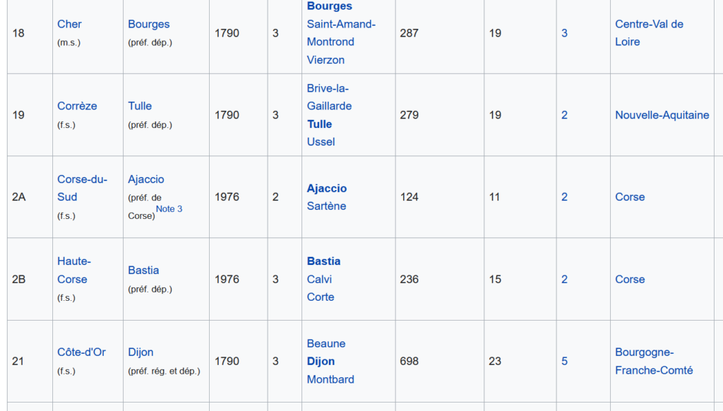
Postal code is better than a city description, as several cities can share the same name in France. For example, there are 4 Saint-Arnoult cities in France, and they have different postal codes:
- In Loir-et-Cher department: 41800.
- In Calvados department: 14800.
- In Oise department: 60220.
- In Seine-Maritime department: 76490.
https://fr.wikipedia.org/wiki/Saint-Arnoult
The real estate depends a lot on the town, so we keep this column.
10 - code_postal
```{r}
# we keep it
```
11 – code_commune column
French: code commune.
English: city code.
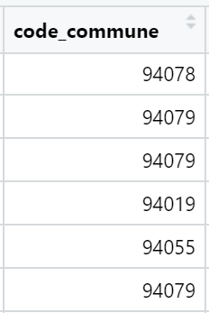
This is an alternative numerical city identifier to code postal. This one is edited by INSEE, which is the French National Institute of Statistics and Economic Studies.
This INSEE identifier looks like a 1:1 mapping rule with the postal code identifier.
In some cases, the postal code is misleading, opposite to the INSEE code.
For example, the city of Saint-Pierre-Laval is in the department Allier, so we could believe its postal code starts with 03.
Indeed, the postal code of Saint-Pierre-Laval is 42620; it belongs to a different department, Loire.
The reason for this is most often a problem of accessibility; when the town or village is tucked away in a valley, it is easier to deliver mail through the valley, even if it means delivering it from another department. And the postal code belongs to the delivering department office.
Despite postal code and INSEE code sometimes could be considered as redundant, we keep both
11 - code_commune
```{r}
# we keep it
```
12 – nom_commune column
French: nom de commune.
English: city name.
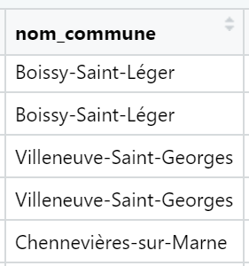
This is the city’s official name, like Créteil, which is the administrative and principal city of the Val-de-Marne department.
Sometimes, the city can be a more precise geographical indicator than the postal code, as several towns might share the same postal code.
For example, the postal code 83186 is shared by 8 towns:
| Postal Code | City | INSEE code ( code_commune column) |
| 83186 | Néoules | 83088 |
| 83186 | Mazaugues | 83076 |
| 83186 | Méounes-lès-Montrieux | 83077 |
| 83186 | Garéoult | 83064 |
| 83186 | La Roquebrussanne | 83108 |
| 83186 | Forcalqueiret | 83059 |
| 83186 | Sainte-Anastasie-sur-Issole | 83111 |
| 83186 | Rocbaron | 83106 |
In conclusion, we keep the city name, as it is sometimes more precise than the postal code.
12 - nom_commune
```{r}
# We keep it
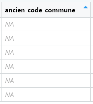
```13 – ancien_code_commune
French: ancien code commune / code postal (5 chiffres).
English: previous postal code (5 digits).
It didn’t happen recently in the department of Val-de-Marne, but some towns may merge in other departments. Usually, small towns benefit from a mutualization effect.
For example, these towns have merged in 2019:
- Contres – ancien_code_commune: 41700
- Feings – ancien_code_commune: 41700
- Fougères-sur-Bièvre – ancien_code_commune: 41700
- Ouchamps – ancien_code_commune: 41700
- Thenay – ancien_code_commune: 41700
They have become the town of Le-Controis-en-Sologne, with an unsurprisingly code_commune: 41700.
Just remember the postal code (code_commune) could have changed.
The merging towns can have different real estate values: for example, Contres is bigger than the others, a local employment area, so the real estate is more expensive than in the other merged towns.
We keep this column as it might sometimes be useful.
Remark: in Val-de-Marne, the complete column is empty.
13 - ancien_code_commune
```{r}
# We keep it
```
14 – ancien_nom_commune
French: ancient nom de commune.
English: previous city name.
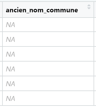
This occurs in the same scenario as in column ancien_code_commune.
In Val-de-Marne, the column is totally empty, as cities in an urban department are usually large and don’t need to merge.
For more rural departments, it might happen. Despite it would have a marginal effect, we keep this data.
14 - ancien_nom_commune
```{r}
# We keep it - could have been removed for Val-de-Marne example
```
15 – code_departement column
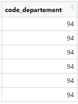
French: code départemental (2 chiffres en Métropole, 3 chiffres en Métropole, la Corse est un cas particulier avec chiffre puis lettre )
English: department code (2 digits in Metropole area, three digits overseas if applicable, Corsica is a specific case with first a digit then a letter)
As we are in Val-de-Marne, the value is always the same, 94.
If there were several departments in the file, one could argue that the department code is already included in the postal code.
For example, Vincennes has a postal code (code_commune) « 94300 », so a column department code (code_department) 94 is redundant. That’s true, but for better understanding, selection, we keep it.
15 - code_departement
```{r}
# We keep it - could have been removed for Val-de-Marne
```
16 – id_parcelle column
French: Identifiant de parcelle cadastrale.
English: Cadastral parcel ID.
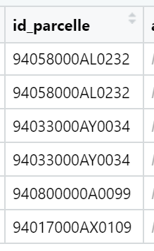
The first characters of this identifier are linked to the city.
The last characters are defining the cadastral parcel, in french parcelle cadastrale:

This is a scan of part of an old administrative document
Part of cadastral plan, Domaine public, https://commons.wikimedia.org/w/index.php?curid=52305536
The parcel ID is unlikely to be helpful. Yes, in theory, it identifies the property. But, in reality, the property could be aggregated or divided.
Finding two sales with the same ID needs a time interval of years or decades. And after decades, the property can evolve so much: for instance, a beautiful house can become a ruin, or a house ruin can be replaced by a building.
Also, the ID parcel probably depends on the city, and for a department unique identifier, some additional consolidation is required.
So we skip this data.
16 - id_parcelle
```{r}
vf <- vf[, id_parcelle:= NULL ]
```
17 – ancien_id_parcelle column
French: Ancien identifiant de parcelle cadastrale.
English: Previous cadastral parcel ID.
As we have decided not to keep the cadastral parcel data, it is logical to not keep the previous cadastral parcel data.
17 - ancien_id_parcelle
```{r}
vf <- vf[, ancien_id_parcelle:= NULL ]
```
18 – numero_volume column
French: Numéro de volume
English: ID of the volume.
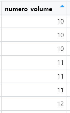
The entries usually are empty. It looks like a subdivision linked to the cadastral parcel.
For the Val-de-Marne file, we don’t keep it.
18 - numero_volume
```{r}
vf <- vf[, numero_volume:= NULL ]
```
Conclusion of the example – part 3
Nine fields have been cleaned.
Some crucial fields like the house/appart square area will be treated in the next post.
Example: deeds of sales – part 4
On progress…