ANN means Artificial Neural Network
ANN is known for its applications in Deep Learning
1 – ANN without hidden layer
This article will be illustrated with R language (installation details: https://vgir.fr/toolbox/ )
Disclaimer
An ANN without a hidden layer has no application. The aim of this chapter is:
- Gentle introduction of the concept
- Analogy of ANN in its less powerful « hidden layer » configuration with an already-seen model
Imaginary scenario
For example, an aeronautic company, Airbing, sells three types of planes:
- Small Size: the airplane P320
- Medium Size: the airplane P330
- Big Size: the airplane P350
The aim is to see if the margin can be explained depending on the number of planes of each type sold each month. If there is a loss, a negative number applies.
Experiences of the scenario
Dataset
Hereunder is a generated dataset for this article corresponding to 10 months:
| P320 sold | P330 sold | P350 sold | Margin (million €) |
| 3 | 3 | 10 | 33 |
| 4 | 2 | 3 | 1 |
| 6 | 7 | 7 | 14 |
| 10 | 4 | 2 | -38 |
| 3 | 8 | 3 | 22 |
| 9 | 5 | 4 | -13 |
| 10 | 8 | 1 | -22 |
| 7 | 10 | 4 | -4 |
| 7 | 4 | 9 | 16 |
| 1 | 8 | 4 | 28 |
An observation is equivalent to a row of the dataset
Explanation of the first row of the dataset in the first month of the series: 3 PP320, 3 P330, and 3 P350 have been sold. The margin is +33 million dollars.
Generalization of the scenario
In a machine-learning context, we have three explicative variables: X1, X2, and X3. So, we are looking to explain variable Y.
Mapping:
| Type of variable | Scenario Name | General Name |
| Input (or explanatory) variable | Plane P320 | X1 |
| Input (or explanatory) variable | Plane P330 | X2 |
| Input (or explanatory) variable | Plane P330 | X3 |
| Output (or target) variable | Margin | Y |
Now we will use the variables X1, X2, X3, and Y.
Modelization of the scenario with an ANN without a hidden layer
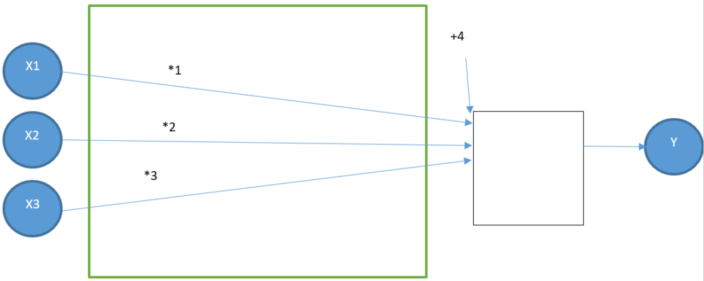
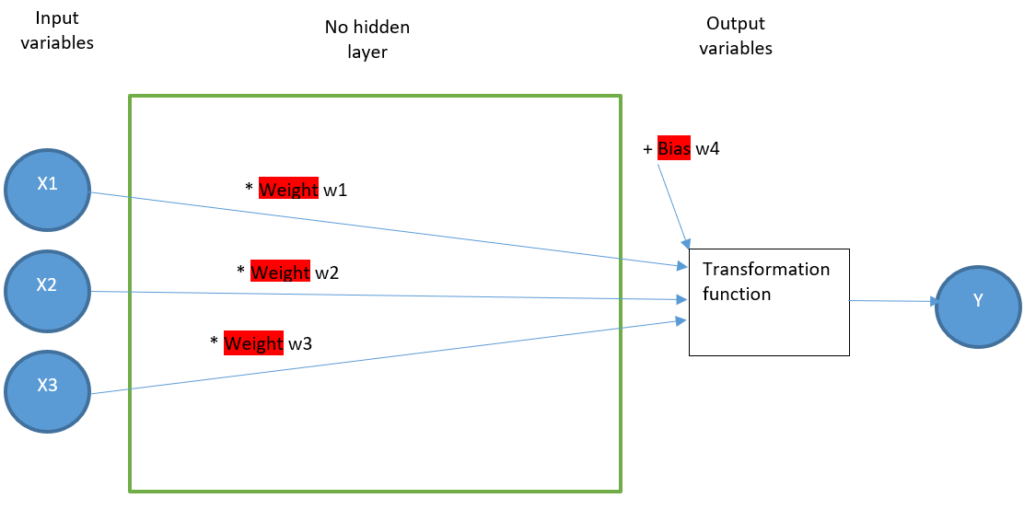
Our first and most possible basic model contains four artificial neurons, represented as yellow circles:
- Three input neurons
- One output neuron
There is no neuron between the input and the output block, so it is called « no hidden layer ». At the very end of this article, you’ll discover two examples with 1 and 2 hidden layers.

This model aims to find four parameters:
- w1
- w2
- w3
- w4
For each row of the dataset, the operations in the figure below give a result close to Y.
When you want to distinguish a real value from an estimated value, add a circumflex accent
Example:
Ŷ : the estimated value
Y : the real value
An example
Let’s illustrate the above figure:
We arbitrarily choose a solution and then do a calculation and check if it fits nicely:
- w1 = 1
- w2 = 2
- w3 = 3
- w4 = 4
We define this model as [1;2;3;4]
The figure is updated accordingly:
The first row is:
| X1 | X2 | X3 | Y |
| 3 | 3 | 10 | 33 |
So, let’s extract its input variables:
| X1 | X2 | X3 |
| 3 | 3 | 10 |
And inject them in the figure:

This model’s result is 43. The real value from the dataset is 33. Hence, we have an error of 10 million between the modelized 43 million and the actual value of 33 million.
Application with R language
Hereunder the « .csv » source file:
Let’s define the working directory
mydirectory <- "C:\\...my_directory..."
setwd(mydirectory)
We’ll work with data tables, so the library is required:
library(data.table)Now we read the source file
data <- fread("ann.csv")# definition of arbitrarily coefficients, the model is called {1,2,3,4}
w1 <- 1
w2 <- 2
w3 <- 3
w4 <- 4
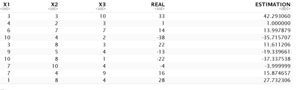
# calcation of estimated values for model {1,2,3,4}
data$ESTIMATION <- data$X1 * w1 + data$X2 * w2 + data$X3 * w3 + w4
# Rename "Y" column into "REAL" for visibility
colnames(data)[colnames(data) == "Y"] <- "REAL"The raw result is:

Metric of the scenario
Why the need for a metric?
To compare the reliability of several models, we need a metric.
The metric is a measurable value indicating the performance of a model
We have many options for determining the global difference; let’s describe three usual metrics:
- Mean percentage error (called MPE)
- Mean absolute percentage error (called MAPE)
- Root mean square error (called RMSE)
How do we interpret the metric?
- If the value is 0, then the model is perfect
- The higher the value, the worse the model
- Between 2 models, the one with the lowest metric is the better
Choice of a metric
Whatever of these three solutions, the aim is to find the parameters w0, w1, w2, and w4 which will minimize the result
Arbitrarily, we use the metric percentage error (called MAPE). Indeed, it is a very classical metric. https://en.wikipedia.org/wiki/Mean_absolute_percentage_error
# Use of a library in order to gain time in the calculation
library(Metrics)
metric <- mape(data$REAL, data$ESTIMATION)
metric

The MAE metric has a result of 4.47, which means we have a terrible global error of 447%.
Definitely, this model [1;2;3;4] with the hereunder coefficients gives an awful result.
- w1 = 1
- w2 = 2
- w3 = 3
- w4 = 4
We hope we can do better. Indeed, ANN aims to find the best coefficients, providing the minimum metric and the minimal error in modelization.
Optimizer of the scenario
Why the need for an optimizer
We know we need to find the values of w1, w2, w3, and w4 coefficients. It is not reasonable to try randomly a large number of values; an infinite number of combinations is possible.
Here, we need an optimizer.
An optimizer is a tool which aim is to find the optimum of a problem.
This optimum can be a minimal or a maximal solution.
It is required when no analytical solution is available (an analytical solution is applied through a precise calculation which provides the best solution.
Optimizer is looking for a numeric solution (a numeric solution may find only a local solution instead of the global solution.), usually through iterations.
We will provide the optimizer with the metric we want to minimize. As seen in the definition, we are still determining whether it will find the global minimum value. The function may be too complex, or the optimizer may not be optimized for this function. At least, it should find a local minimum.
We arbitrarily chose the optim function in the R language as an optimizer. This is a simple optimizer, which does not suit deep learning. Indeed, we only need to understand the concept of ANN and whether any optimizer is suitable.
First, we define the function to optimize.
Beware of the new paradigm
– Before, in the example w1, w2, w3, w4 were fixed values
– Now w1, w2, w3, w4 become some variables, while X1, X2, X3 are fixed
Let’s name it fmetric, and we know it depends on {w1,w2,w3,w4}
Remember, we’ll need to minimize fmetric, as we want w1, w2, w3, and w4 to make the error as small as possible.
Previously, we have written metric <- mape(data$REAL, data$ESTIMATION). data$REAL is known. We need to calculate data$ESTIMATION depending on {w1,w2,w3,w4}
Let’s detail data$ESTIMATION:
| X1 | X2 | X3 | ESTIMATION |
| 3 | 3 | 10 | W1*3+W2*3+W3*10+W4 |
| 4 | 2 | 3 | W1*4+W2*2+W3*3+W4 |
| 6 | 7 | 7 | … |
| 10 | 4 | 2 | … |
| 3 | 8 | 3 | … |
| 9 | 5 | 4 | … |
| 10 | 8 | 1 | … |
| 7 | 10 | 4 | … |
| 7 | 4 | 9 | … |
| 1 | 8 | 4 | … |
One last thing: the function optim is working with an input vector. Instead of four input parameters w1, w2, w3, w4, we are providing it one vector w of four values
We are ready to code everything above in R:
# definition of the function fmetric. It depends on the vector w, containing 4 numeric values w[1],  w[2],  w[3],  w[4],
fmetric <- function(w) {
  # in case of debugging, why not giving another name for the data table
  tempdata <- data
  # calculation of all estimations values
  tempdata$ESTIMATION <- w[1] * tempdata$X1 + w[2] * tempdata$X2 + w[3] * tempdata$X3 + w[4]
  # the function returns the MAPE
  return(mape(tempdata$REAL, tempdata$ESTIMATION))
  }
Let’s check the result is the same for {1,2,3,4}
myweight <- c(1,2,3,4)
fmetric(myweight)
We have the same result, and we assume fmetric is correct. We are ready to optimize it, and the R function optim requires:
- The starting points w1, w2, w3, w4. We have no idea how to choose some good initial points. Hence, arbitrarily, we chose {0,0,0,0}
- The function fmetric to optimize
- By default, optim is minimizing; it’s what we seek
set.seed(123)
optim( c(0,0,0,0), fmetric)
With the values
w1 = -5.57
w2 = 0.84
w3 = 4.98
w4 = 6.64
Let’s find the estimations according to the weights:
tempdata <- data
tempdata$ESTIMATION <- tempdata$X1 * result_par[1] + tempdata$X2 * result_par[2] + tempdata$X3 * result_par[3] +  result_par[4]
tempdata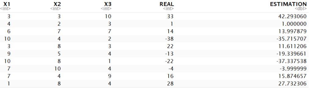
mape(tempdata$REAL, tempdata$ESTIMATION)
Analysis of the no-hidden layer ANN
Disclaimer: with no hidden layer, the analysis is oversimplified
Remind this article is a ramp-up before going deeper into the complexity of the ANN
Considering the starting hypothesis is:
This means the estimated value is calculated with
Yestimated = W1*X1+W2*X2+W3*X3+W4
Yestimated = -5.58*X1+0.84*X2+4.98*X3+6.64
The explanation given by the model is:
- 5.58 million€ loss per plane P320 sold each month.
- 0.84 million€ gain per plane P330 sold each month.
- 4.98 million€ gain per plane P340 sold each month.
- 6.64 million€ fixed gain each month: some fixed training, certification, maintenance, earned by Airbing?
We managed to have a global accuracy of 20.2%.
For this very very light ANN, the model is explainable.
A feeling of « déjà vu »?
Instead of MAPE metric, if you choose the RSE (Root Square error) metric, translate:
- weight into coefficient
- bias into intercept
And then you have a linear regression, described in this article:
https://vgir.fr/linear-regression/
Indeed, the linear regression provides an analytical solution:
- It calculates in one time the solution.
- It provides the best solution.
The no-hidden layer has provided a numerical solution
- It calculates many solutions with many iterations.
- At the last iteration, it is not sure to find the best solution.
Indeed, why is applying a solution less performant than the linear regression?
Remember this example has no hidden layer. We will increase the complexity
ANN is complex. An adequate learning curve is required:

2 – One ANN with 1 hidden layer
As you know now how an ANN without a hidden layer has been built, we create an ANN with seven artificial neurons including one hidden layer:
- Three input neurons
- Three hidden layer neurons
- One output neuron
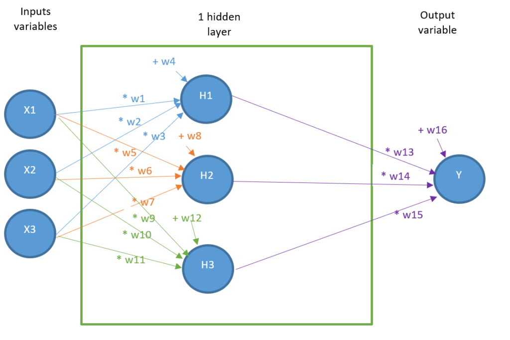
The aim of this model is now to find 16 parameters:
| w1 | w5 | w9 | w13 |
| w2 | w6 | w10 | w14 |
| w3 | w7 | w11 | w15 |
| w4 | w8 | w12 | w16 |
Such that, for each row of the dataset, the operations in the hereunder figure give a result close to Y
For example, we arbitrarily choose a solution and then do a calculation and check if it fits nicely:
Let’s illustrate the above figure:
| w1=1 | w5=-1 | w9=2 | w13=-2 |
| w2=2 | w6=2 | w10=-3 | w14=2 |
| w3=-1 | w7=1 | w11=2 | w15=-1 |
| w4=-2 | w8=1 | w12=1 | w16=1 |
We define this model as [1,2,-1,-2,-1,2,1,1,2,-3,2,1,-2,2,-1,1]
Reminder: the dataset is
| P320 sold | P330 sold | P350 sold | Margin (million €) |
| 3 | 3 | 10 | 33 |
| 4 | 2 | 3 | 1 |
| 6 | 7 | 7 | 14 |
| 10 | 4 | 2 | -38 |
| 3 | 8 | 3 | 22 |
| 9 | 5 | 4 | -13 |
| 10 | 8 | 1 | -22 |
| 7 | 10 | 4 | -4 |
| 7 | 4 | 9 | 16 |
| 1 | 8 | 4 | 28 |
We extract the first row input variables:
| X1 | X2 | X3 |
| 3 | 3 | 10 |
First, we set the weights:

Then, the intermediate calculations: for example, the first intermediate neuron has a value of 3*1 + 3*2 + 10*-1 -2 = -3

Then the final value: for instance, the output neuron has the value -3*-2 + 12*2 + 18*-1 +1 = 13

Hence the estimated value of the model [1,2,-1,-2,-1,2,1,-1,2,-3,2,1,-2,2,-1,1] is 13 instead of a real value of 33 million €
The MAPE error for this value is (13-33)/33 = 60.6%.
Application with R language
Hereunder the “.csv” source file:
Let’s define the working directory:
mydirectory <- "C:\\...my_directory..."
setwd(mydirectory)
We’ll work with data tables, so the library is required:
library(data.table)Now we read the source file:
data <- fread("ann.csv")# definition of arbitrarily coefficients, the model is called [1,2,-1,-2,-1,2,1,-1,2,-3,2,1,-2,2,-1,1]
# we directly use an vector, in order not to create 16 different variable
w <- c(1,2,-1,-2,-1,2,1,-1,2,-3,2,1,-2,2,-1,1)
tempdata <- data
# calcation of estimated values for model [1,2,-1,-2,-1,2,1,-1,2,-3,2,1,-2,2,-1,1]
tempdata$H1 <- ( tempdata$X1 * w[1] + tempdata$X2 * w[2] + tempdata$X3 * w[3] + w[4] )
tempdata$H2 <- ( tempdata$X1 * w[5] + tempdata$X2 * w[6] + tempdata$X3 * w[7] + w[8] )
tempdata$H3 <- ( tempdata$X1 * w[9] + tempdata$X2 * w[10] + tempdata$X3 * w[11] + w[12] )
tempdata$ESTIMATION<- ( tempdata$H1 * w[13] + tempdata$H2 * w[14] + tempdata$H3 * w[15] + w[16] )
# Rename "Y" column into "REAL" for visibility
colnames(tempdata)[colnames(tempdata) == "Y"] <- "REAL"
Choice of a metric
We keep the same metric than in zero hidden layer: the MAPE (Moving Average Percentage Error)
We check the individual MAPE:
tempdata$MAPE <- abs( (tempdata$REAL - tempdata$ESTIMATION) / tempdata$REAL )
library(Metrics)
metric <- mape(tempdata$REAL, tempdata$ESTIMATION)
metric
Optimizer of the scenario
We keep the optim function from the R language. As we will jump from 4 variables to 16 variables:
- The optimizer will need more time.
- The optimizer is more likely to find a sub-optimal solution.
Remember, we’ll need to minimize fmetric, as we want w1…w16 such that error is as small as possible.
Previously, we have written metric <- mape(data$REAL, data$ESTIMATION). data$REAL is known. We need to calculate data$ESTIMATION depending on {w1,w2,w3,w4,w5,w6,w7,w8,w9,w10,w11,w12,w13,w14,w15,w16}
Let’s detail data$ESTIMATION:
| X1 | X2 | X3 | ESTIMATION |
| 3 | 3 | 10 | (W1*3+W2*3+W3*10+W4)*W13 + (W5*3+W6*3+W7*10+W8)*W14 + (W9*3+W10*3+W11*10+W12)*W15 + W16 |
| 4 | 2 | 3 | (W1*4+W2*2+W3*3+W4)*W13 + (W5*4+W6*2+W7*3+W8)*W14 + (W9*4+W10*2+W11*3+W12)*W15 + W16 |
| 6 | 7 | 7 | … |
| 10 | 4 | 2 | … |
| 3 | 8 | 3 | … |
| 9 | 5 | 4 | … |
| 10 | 8 | 1 | … |
| 7 | 10 | 4 | … |
| 7 | 4 | 9 | … |
| 1 | 8 | 4 | … |
We are ready to code everything above in R:
# definition of the function fmetric. It depends on the vector w, containing 4 numeric values w[1],  w[2],  w[3],  w[4],
fmetric <- function(w) {
  # in case of debugging, why not giving another name for the data table
tempdata <- data
  # calculation of all estimations values
tempdata$H1 <- ( tempdata$X1 * w[1] + tempdata$X2 * w[2] + tempdata$X3 * w[3] + w[4] )
tempdata$H2 <- ( tempdata$X1 * w[5] + tempdata$X2 * w[6] + tempdata$X3 * w[7] + w[8] )
tempdata$H3 <- ( tempdata$X1 * w[9] + tempdata$X2 * w[10] + tempdata$X3 * w[11] + w[12] )
tempdata$ESTIMATION<- ( tempdata$H1 * w[13] + tempdata$H2 * w[14] + tempdata$H3 * w[15] + w[16] )
  # the function returns the MAPE
  return(mape(tempdata$REAL, tempdata$ESTIMATION))
  }
Let’s check the result is same for the model [1,2,-1,-2,-1,2,1,-1,2,-3,2,1,-2,2,-1,1]
colnames(tempdata)[colnames(tempdata) == "Y"] <- "REAL"
myweight <- c(1,2,-1,-2,-1,2,1,-1,2,-3,2,1,-2,2,-1,1)
fmetric(myweight)
We have the same result; we assume fmetric is correct. We are ready to optimize it, and the R function optim requires:
- starting points w1,w2,w3,w4,w5,w6,w7,w8,w9,w10,w11,w12,w13,w14,w15,w16 . Right now, we have no clue for choosing some good initial points. Hence, arbitrarily, we chose {0,0,0,0, 0,0,0,0,0,0,0,0,0,0,0,0}
- the function fmetric to optimize
- by default, optim is minimizing, it’s what we seek
set.seed(123)
optim( rep(0,16), fmetric)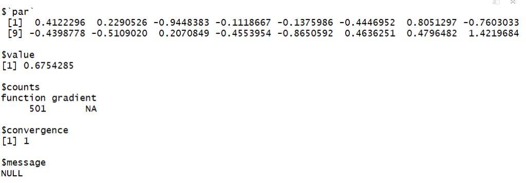
Bad luck, the error is 67.5%, it is worst than with no-hidden layer which is 20.1%!
Maybe it is linked to the starting point? Let’s try two others:
set.seed(123)
optim( rep(1,16), fmetric)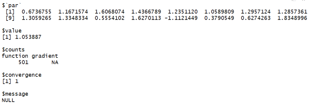
set.seed(123)
optim( rep(-1,16), fmetric)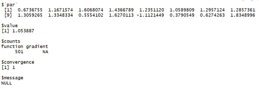
With the starting points (1,1,1,1,1,1,1,1,1,1,1,1,1,1,1,1) and (-1,-1,-1,-1,1,1-,-1,-1,-1,-1,-1,-1,-1,-1,-1,-1) it is even worst.
Let’s have an overview:
In theory our model with 1 hidden layer cannot be worst than our model with no hidden layer.
Explanation of reality different from theory:
Set :
- w1 = 1 / w2 = 0 / w3 = 0 / w4 =0 => H1 as same value than X1
- w5 = 0 / w6 = 1 / w7 = 0 / w8 =0 => H2 as same value than X2
- w9 = 0 / w10 = 0 / w11 = 1 / w12 =0 => H3 as same value than X3
It means this is like:
With the transcodification:
- w13[1-layer] becomes w1[0-layer]
- w14[1-layer] becomes w2[0-layer]
- w15[1-layer] becomes w3[0-layer]
- w15[1-layer] becomes w3[0-layer]
Our model with no layer is a sub-element of our model with 1 layer.
Indeed, the model with 1 hidden layer proposes maybe calculation combinations, including the the ones from the model without hidden layer
Hence, in theory, the model with one hidden layer is at least as performing as the model with two hidden layers.
Why a model with more layers can be less performing than its reference model?
The explanation is inside the optimizer: the more variables, the less effective. It’s a classical optimization issue.
Then, for ANNand indeed for deep learning, the issue is finding performant optimizers. It’s why you need to find a suitable package with a good optimizer when applied to ANN.
Spoiler: this is very complex to develop a good optimizer for ANN.
Indeed, it’s why there are so many packages available, like:
- Tensor Flow
- Keras
- Theano
- Scikit-learn
- PyTorch
There are many ways for starting an optimizer package, many ways to improve it, and sometimes it comes to a dead-end, needing a fresh start.
It’s why when applied to different ANN, the result of the packages can be totally different, and why it can be an option to test many of them.
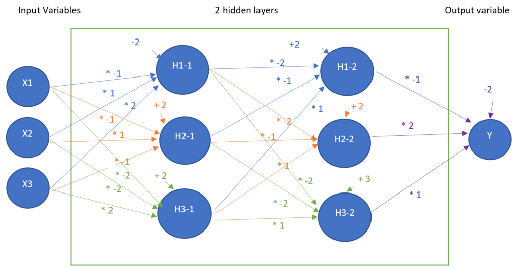
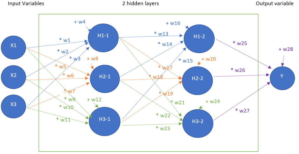
3 – ANN with 2 hidden layers
Now, we add one hidden and create an ANN with 2 hidden layers, meaning 10 artificial neurons in this example
- Three input neurons
- Three + three hidden layer neurons
- One output neuron

The aim of this model is now to find 16 parameters:
| w1 | w5 | w9 | w13 | w17 | w21 | w25 |
| w2 | w6 | w10 | w14 | w18 | w22 | w26 |
| w3 | w7 | w11 | w15 | w19 | w23 | w27 |
| w4 | w8 | w12 | w16 | w20 | w24 | w28 |
Such that, for each row of the dataset, the operations in the hereunder figure, give a result close to Y
An example
We choose arbitrarily a solution, and then do a calculation and check if it fits well:
| w1=-1 | w5=-1 | w9=-2 | w13=-2 | w17=-2 | w21=-2 | w25=-1 |
| w2=1 | w6=1 | w10=-2 | w14=-1 | w18=-1 | w22=-2 | w26=2 |
| w3=2 | w7=-1 | w11=2 | w15=1 | w19=1 | w23=1 | w27=1 |
| w4=-2 | w8=2 | w12=2 | w16=2 | w20=2 | w24=3 | w28=-2 |
Let’s illustrate the above figure:
We define this model as Model 2-0.
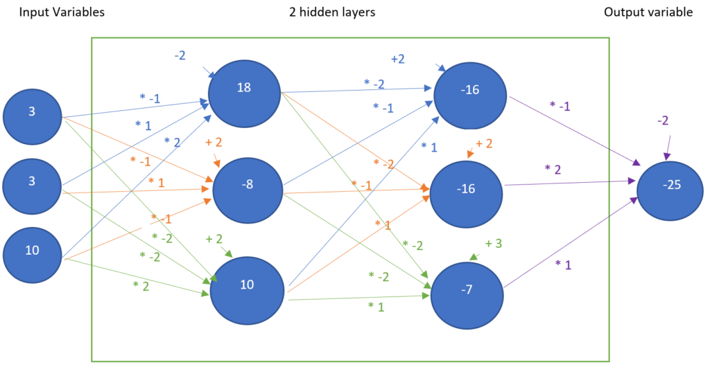
We extract the first row input variables:
| X1 | X2 | X3 |
| 3 | 3 | 10 |
First, we set the weights:
Calculation of the first row:
Calculation with R:
# we directly use an vector, in order not to create 28 different variables
w <- c( -1, 1, 2, -2,
        -1, 1, -1, 2,
        -2, -2, 2, 2,
        -2, -1, 1, 2,
        -2, -1, 1, 2,
        -2, -2, 1, 3,
        -1, 2, 1, -2)
tempdata <- data
# calcation of estimated values for model [1,2,-1,-2,-1,2,1,-1,2,-3,2,1,-2,2,-1,1]
tempdata$H11 <- ( tempdata$X1 * w[1] + tempdata$X2 * w[2] + tempdata$X3 * w[3] + w[4] )
tempdata$H21 <- ( tempdata$X1 * w[5] + tempdata$X2 * w[6] + tempdata$X3 * w[7] + w[8] )
tempdata$H31 <- ( tempdata$X1 * w[9] + tempdata$X2 * w[10] + tempdata$X3 * w[11] + w[12] )

tempdata$H12 <- ( tempdata$H11 * w[13] + tempdata$H21 * w[14] + tempdata$H31 * w[15] + w[16] )
tempdata$H22 <- ( tempdata$H11 * w[17] + tempdata$H21 * w[18] + tempdata$H31 * w[19] + w[20] )
tempdata$H32 <- ( tempdata$H11 * w[21] + tempdata$H21 * w[22] + tempdata$H31 * w[23] + w[24] )

tempdata$ESTIMATION<- ( tempdata$H12 * w[25] + tempdata$H22 * w[26] + tempdata$H32 * w[27] + w[28] )

# Rename "Y" column into "REAL" for visibility
colnames(tempdata)[colnames(tempdata) == "Y"] <- "REAL"
What is the error according to the MAPE metric?
metric <- mape(tempdata$REAL, tempdata$ESTIMATION)
metric
Optimizer of the scenario
We keep the optim function from the R language. Now we have 28 variables instead of 16 variables.
The risk of performance degradation is indeed greater.
Remember, we’ll need to minimize fmetric, as we want w1…w28 such that error is as small as possible.
Previously we have written metric <- mape(data$REAL, data$ESTIMATION). data$REAL is known. We need to calculate data$ESTIMATION depending on {w1,w2,w3,w4,w5,w6,w7,w8,w9,w10,w11,w12,w13,w14,w15,w16,w17,w18,w19,w20,w21,w22,w23,w24,w25,w26,w27,w28}
Let’s detail data$ESTIMATION:
| X1 | X2 | X3 | ESTIMATION |
| 3 | 3 | 10 | W25*(W13*(W1*3+W2*3+W3*10+W4)+W14* (W5*3+W6*3+W7*10+W8)+W15* (W9*3+W10*3+W11*10+W12)+W16)+ W26*( W17*(W1*3+W2*3+W3*10+W4)+W18* (W5*3+W6*3+W7*10+W8)+W19* (W9*3+W10*3+W11*10+W12)+W20)+ W27*( W21*(W1*3+W2*3+W3*10+W4)+W22* (W5*3+W6*3+W7*10+W8)+W23* (W9*3+W10*3+W11*10+W12) +W24)+ W28 |
| 4 | 2 | 3 | … |
| 6 | 7 | 7 | … |
| 10 | 4 | 2 | … |
| 3 | 8 | 3 | … |
| 9 | 5 | 4 | … |
| 10 | 8 | 1 | … |
| 7 | 10 | 4 | … |
| 7 | 4 | 9 | … |
| 1 | 8 | 4 | … |
Yes, I know, the equation becomes quite long. It could be develop, without any real comprehension gain.
We are ready to code everything above in R:
# definition of the function fmetric. It depends on the vector w, containing 28 numeric values w[1],  w[2],  w[3],  w[4],...w[28]
fmetric <- function(w) {
  # in case of debugging, why not giving another name for the data table
tempdata <- data
# calcation of estimated values for model [1,2,-1,-2,-1,2,1,-1,2,-3,2,1,-2,2,-1,1]
tempdata$H11 <- ( tempdata$X1 * w[1] + tempdata$X2 * w[2] + tempdata$X3 * w[3] + w[4] )
tempdata$H21 <- ( tempdata$X1 * w[5] + tempdata$X2 * w[6] + tempdata$X3 * w[7] + w[8] )
tempdata$H31 <- ( tempdata$X1 * w[9] + tempdata$X2 * w[10] + tempdata$X3 * w[11] + w[12] )

tempdata$H12 <- ( tempdata$H11 * w[13] + tempdata$H21 * w[14] + tempdata$H31 * w[15] + w[16] )
tempdata$H22 <- ( tempdata$H11 * w[17] + tempdata$H21 * w[18] + tempdata$H31 * w[19] + w[20] )
tempdata$H32 <- ( tempdata$H11 * w[21] + tempdata$H21 * w[22] + tempdata$H31 * w[23] + w[24] )

tempdata$ESTIMATION<- ( tempdata$H12 * w[25] + tempdata$H22 * w[26] + tempdata$H32 * w[27] + w[28] )
  # the function returns the MAPE
  return(mape(tempdata$REAL, tempdata$ESTIMATION))
  }
Checking the metric with the previous example:
colnames(data)[colnames(data) == "Y"] <- "REAL"
myweight <-
     c( -1, 1, 2, -2,
        -1, 1, -1, 2,
        -2, -2, 2, 2,
        -2, -1, 1, 2,
        -2, -1, 1, 2,
        -2, -2, 1, 3,
        -1, 2, 1, -2)
fmetric(myweight)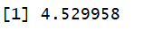
set.seed(123)
optim( rep(0,28), fmetric)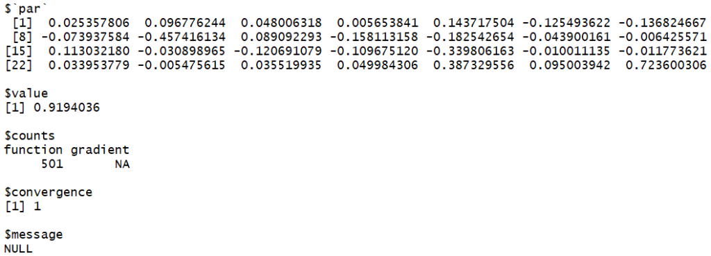
Again, the model with two hidden layers, 92% MAPE error, is disappointing compared to zero hidden layer, 20%.
Nevertheless, there is a gain compared to the 1-hidden layer, 168%.
The reasons are the same as one hidden layer: the more variables, the less compelling. It’s again a classical optimization issue.
Interpretation of the results with 2 hidden layers
Here you get the 28 W1…W28 parameters:
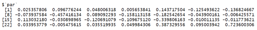
It means the estimation of Y is equal to
Y estimated =
W25*(W13*(W1*3+W2*3+W3*10+W4)+W14* (W5*3+W6*3+W7*10+W8)+W15* (W9*3+W10*3+W11*10+W12)+W16)+
W26*( W17*(W1*3+W2*3+W3*10+W4)+W18* (W5*3+W6*3+W7*10+W8)+W19* (W9*3+W10*3+W11*10+W12)+W20)+
W27*( W21*(W1*3+W2*3+W3*10+W4)+W22* (W5*3+W6*3+W7*10+W8)+W23* (W9*3+W10*3+W11*10+W12) +W24)+
W28
With
W1= 0.025357806
W2 = 0.096776244
…
W28 = 0.723600306
As a conclusion, it is not possible to humanly interpret the results with ANN with 2 hidden layers.

We only have an estimation.
After adding only a couple of hidden layers, ANN becomes a black box. This can be an issue:
- when money is invested: the less understanding by the business team, the less confidence
- it could be required legally or asked by the customer to understand the model. For example, why a credit is denied by a bank?
Conclusion
The aim of these two articles about ANN was to point out:
- It requires complex calculation
- It is a black box about understanding