Starting with the dice example
If you roll ten times a die D-6, can you predict the average value of these ten rolls?
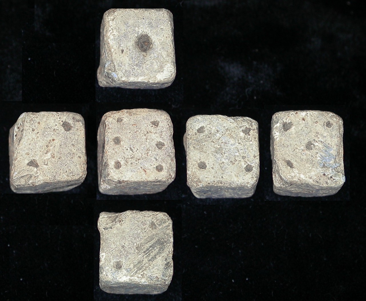
https://commons.wikimedia.org/wiki/File:9BFE00_-roman_lead_die_(FindID_103936).jpg
The first method could be statistics
There is:
- A probability of 1/6 to get a 1
- A probability of 1/6 to get a 2
- A probability of 1/6 to get a 3
- A probability of 1/6 to get a 4
- A probability of 1/6 to get a 5
- A probability of 1/6 to get a 6
Then, the average value is
1/6 * 1 + 1/6 * 2 + 1/6 * 3 + 1/6 * 4 + 1/6 * 5 + 1/6 * 6 =
1/6* (1 + 2 + 3 + 4 + 5 + 6) =
1/6 * 21 =
3.5
A second method could be to simulate 10 dice rolls with a program
We use R language:
# We want reproducible dice
set.seed(5)
# Simulate the rolls
# The possible values are 1,2,3,4,5,6
# Size is my number of rolls
# Replace is TRUE, meaning if a value is rolled, it be can rolled again
my_rolls <- sample(x = c(1,2,3,4,5,6), 10, replace = TRUE, )
print(my_rolls)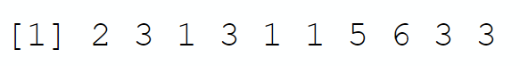
# Calculate the average value
my_mean <- mean(my_rolls)
print(my_mean)
Third method: indeed a real test, not a prediction

By the way, I got an average of 3 when physically rolling ten dice!
Concept of Agent-Based Model
The first method, the statistic one, can be considered a macro-level model, as the dice were considered a general entity with a global behavior.
The second method used in the simulation is an agent-based model. We wrote a simulation in R language in which each die was « living its own life independently. » Thus, each die was an agent.
The dice simulation can be considered a micro-level model, as each dice was considered separately and has its own independent behavior. We had to simulate each die separately.
Now we will shorten Agent-Based Model by ABM
NetLogo Software
Introduction
NetLogo is a cost-free software and an ABM language editor with many library examples.
Wilensky, U. (1999). NetLogo. http://ccl.northwestern.edu/netlogo/. Center for Connected Learning and Computer-Based Modeling, Northwestern University, Evanston, IL.
Installation
It is described here: https://vgir.fr/toolbox/
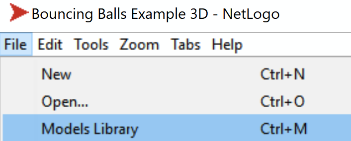
Running a library
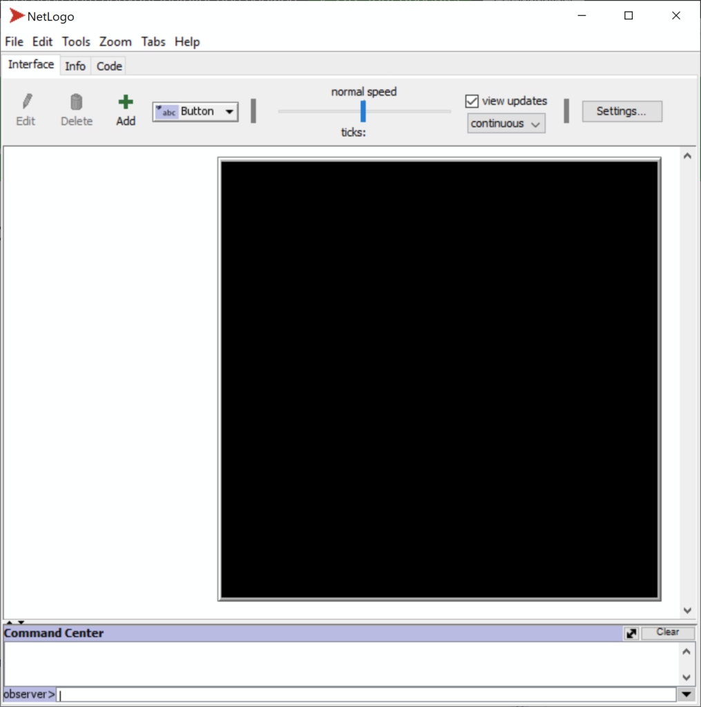
Run « Netlogo »,

The homepage is:
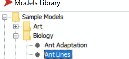
Libraries
Hundreds of libraries are available:

First model: The ant lines
This model is from:
Wilensky, U. (1997). NetLogo Ant Lines model. http://ccl.northwestern.edu/netlogo/models/AntLines. Center for Connected Learning and Computer-Based Modeling, Northwestern University, Evanston, IL.
The short description is:
This project models the behavior of ants following a leader towards a food source. The leader ant moves towards the food along a random path; after a small delay, the second ant in the line follows the leader by heading directly towards where the leader is located. Each subsequent ant follows the ant ahead of it in the same manner.
Quote from Wilensky, U.
The model aims to define the shape of the ant line
Let’s run the « Ant lines » model:
The long description is:
http://ccl.northwestern.edu/netlogo/models/AntLines
The library path is:
The video result is:
After watching the video, you notice the sequence: The model is calculated step after step. The NetLogo word for « step » is « tick. »
At each step/tick:
- The next position of the first ant, called leader ant, is calculated
- The next position of the second ant is calculated
- The next position of the third ant is calculated
- …
- The next position of the last ant is calculated
- A new ant is added to the ant line
- The next position of the first ant is calculated
Also, each ant behaviors independently, with a mixture of randomness and social attributes.
Consequently, each ant is an agent.
You have understood the ABM concept!
Initialization parameters
There are three initialization parameters for the Ant Line ABM:
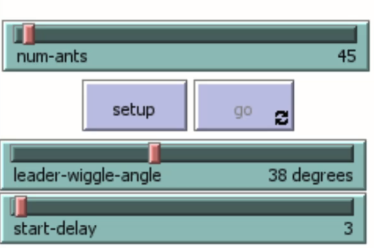
- The number of ants
- The possible wigger angle of the leader ant
- The start delay of ants following the leader
In the next paragraph, we will discover these initialization parameters can have a crucial influence.
Second model: the Wolf Sheep Predation model
This model is from:
Wilensky, U. (1997). NetLogo Wolf Sheep Predation model. http://ccl.northwestern.edu/netlogo/models/WolfSheepPredation. Center for Connected Learning and Computer-Based Modeling, Northwestern University, Evanston, IL.
The short description is
This model explores the stability of predator-prey ecosystems. Such a system is called unstable if it tends to result in extinction for one or more species involved. In contrast, a system is stable if it tends to maintain itself over time, despite fluctuations in population sizes.
Quote from Wilensky, U.
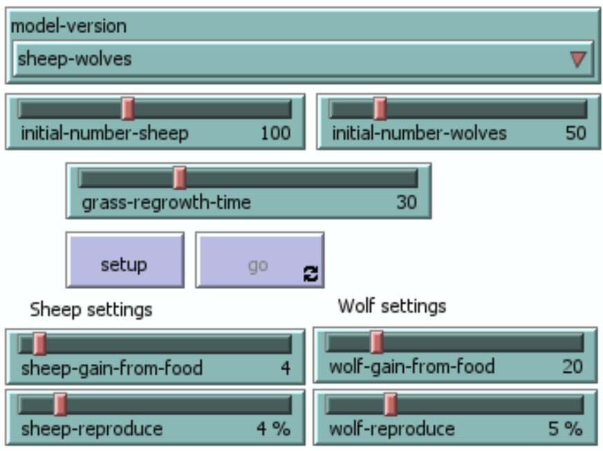
This example has been chosen because there are many initialization parameters with potentially incredible impact:
- Limited or unlimited grass
- The initial number of sheep
- The initial number of wolves
- Grass regrowth time
- Sheep gain from food
- Wolf gain from food
- Sheep reproduction rate
- Wolf reproduction rate
And according to these parameters, you can get three main scenarios:
- The wolves rule the world (and finally, they starve to death)
- The sheep rule the world
- The sheep and the wolves share the world
As there are random processes in the agent behaviors and NetLogo is not reproducing the random effects, the runs are not reproducible! So, you won’t get the same result as I do with the same initialization parameters. Indeed, if you run twice with the same parameter, you will also have different agent behaviors.
1. The wolves rule the world (and finally, they starve to death)
This scenario is quite easy to understand as a summary:
- The wolves reproduce quickly.
- As they become numerous, they eat more and more sheep.
- The sheep population decreases until zero.
- When the wolves have no more game, they eventually all starve to death.
Indeed, as all the species are extinct at the end, the real winner is the grass!
2. The sheep rule the world
The summary
- Both sheep and wolf populations grow.
- But sheep grow faster.
- It means more game for the wolves who raise a lot.
- But the wolves eat too many sheep, and the wolf population decline.
- Then, it becomes difficult for the wolves to find games: many of them starve to death.
- A couple of sheep manage to escape the wolves. Please note that as the path of sheep and the path of wolves, there is a probability that a couple is lucky, meets, and eats the remaining sheep. In this alternative scenario, the wolves would have ultimately become the ultimate animal species!
- Remained a couple of sheep, and all the wolves starved to death: as the sheep have no more predators, and as the grass parameter has been set as unlimited, hence the sheep reproduce and conquer the world.
The video result:
3. The sheep and wolves have a balance and coexist
The summary:
- The initial parameters are that sheep have a high reproducibility rate, and wolves gain a lot of energy from eating food.
- There are fluctuations, sometimes with more wolves and sometimes with more sheep, but a balance has been found, and the two species coexist.
- The coexistence may not be forever:
- Imagine a scenario where all the sheep, due to the random path, are unlucky and meet wolves: then the sheep would become extinct, as already seen.
- Imagine a scenario in which all the wolves, due to the random path, are unlucky and don’t meet sheep: the wolves would become extinct, as already seen.
The video result is:
Remarks from this Wolf-Sheep model
We can mention:
- ABM includes many random effects, as macro-models usually take probability into account.
- Hence, ABM can be very useful for human simulations.
- The macro model usually provides a unique result with the same initial parameters. An agent-based model can include random actions in the agent, and the ABM results can vary according to the different runs.
- So, ABM can estimate its robustness by repeatedly running and comparing the same model.
- The ABM allows us to trace each agent, get a better analysis, and maybe improve the model.
- The ABM needs to calculate each agent at each step: this may require a lot of calculation power, maybe too much.
- And the calculation for each step can be very complex to program.
NetLogo 3D
Netlogo has also a program that works in 3D:
; To the extent possible under law, Uri Wilensky has waived all
; copyright and related or neighboring rights to this model.
The video result is as follows:
Conclusion of Netlogo
Running some models is a better way to understand Agent-based models. Netlogo, with its model libraries, is the ideal learning tool.
We have discovered scenarios where ABM is more powerful than macro-model, because of:
- Complexity
- Sometimes, it is mandatory to examine the individual agent behaviors, such as the ant lines.
- Need to check the importance of parameters and randomness
- How a macro model would guess or explain the three outcomes, sheep win/wolves win/sheep and wolves coexist, due to explanation variables and/or randomness.
Unfortunately, the ABM is more complex to code and usually requires more calculation power, which might be a show-stopper.
Now you have a better idea of an ABM and its pros and cons.
Developing our own ABM: The Plant 4-Species Competition
Remark: this ABM has been developed during my DSTI Master of Science
The model aim
It analyzes the evolution of four plant species over time.
Will the four plants reproduce quickly?
Will they share the field, or will one exterminate the others ?
How do the plants evolve according to favorable or unfavorable soil?
The Netlogo background: the field
The background is a field, a square of 16*16 soil units.
A field unit is called a patch
NetLogo glossary
The plant attributes
Each soil patch has two properties:
- moisture
- Value « 0 » if the soil is dry
- Value « 1 » if the soil is wet
- ph
- Value « 0 » if the soil is neutral
- Value « 1 » if the soil is acid
The timeline
This is in a tropical area; hence, there is no season. The time unit will be a month.
A time unit is called a tick
NetLogo Glossary
The agents: the plants
On the soil, plants can grow and reproduce.
We will follow the destiny of the plant ecosystem on the soil through time.
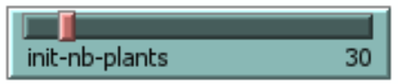
At the beginning of the model, there are some plants generated: the number is an initialization variable:
Each plant has 4 properties:
- lifepoints:
- it’s an unlimited floating number, fluctuating, and if it reaches 0, then the plant dies
- age: in months, as each tick represents one month
- ph: « 0 » if the plant likes neutral soil, « 1 » if the plant likes acid soil
- moisture: « 0 » if the plant likes dry soil, « 1 » if the plant likes wet soil
There are some constraints for the plants, which are also initialization variables:
- The maximum growth age for a spontaneous increase in energy
Some remarks:
- The maximum number of plants on the field is 600
The life cycle of each plant on each tick contains two parts:
- The plant may grow
- The plant may expand
- The plant may die
The plant growth
When the plant is young, it naturally grows, gaining one life point each month. But it loses this prime when the plant reaches its maximum growing age.
Each month, each plant always gets prime and/or penalty according to its compatibility with the hereunder soil:
- There is a ph prime that is an initialization parameter in the following cases:
- If the plant likes acid, and the soil is acid
- If the plant likes neutral, and the soil is neutral
- There is a ph penalty that is an initialization parameter in the following cases:
- If the plant likes acid and the soil is neutral
- If the plant likes neutral, and the soil is acid
- There is a moisture prime that is an initialization parameter in the following cases:
- If the plant likes wet, and the soil is wet
- If the plant likes dry, and the soil is dry
- There is a ph penalty that is an initialization parameter in the following cases:
- If the plant likes wet, and the soil is dry
- If the plant likes dry, and the soil is wet
The primes and penalties are initialization and customizable parameters
The plant expansion
At each tick, check if the plant’s life points reach the minimum for expansion ( initialization and customizable parameter). If yes, the plant loses 16 life points. It gives birth to 8 sowings in all directions around the mother plant. Each new sowing receives two life points.
The plant fight
If plants share the same soil (patch), they will fight
With the expansion, two or more plants may share the same soil: they will each tick fight to dominate this soil patch and lose life points.
The plant death
The plant may die
If the life points are 0 or below 0, the plant dies.
Last details of the model
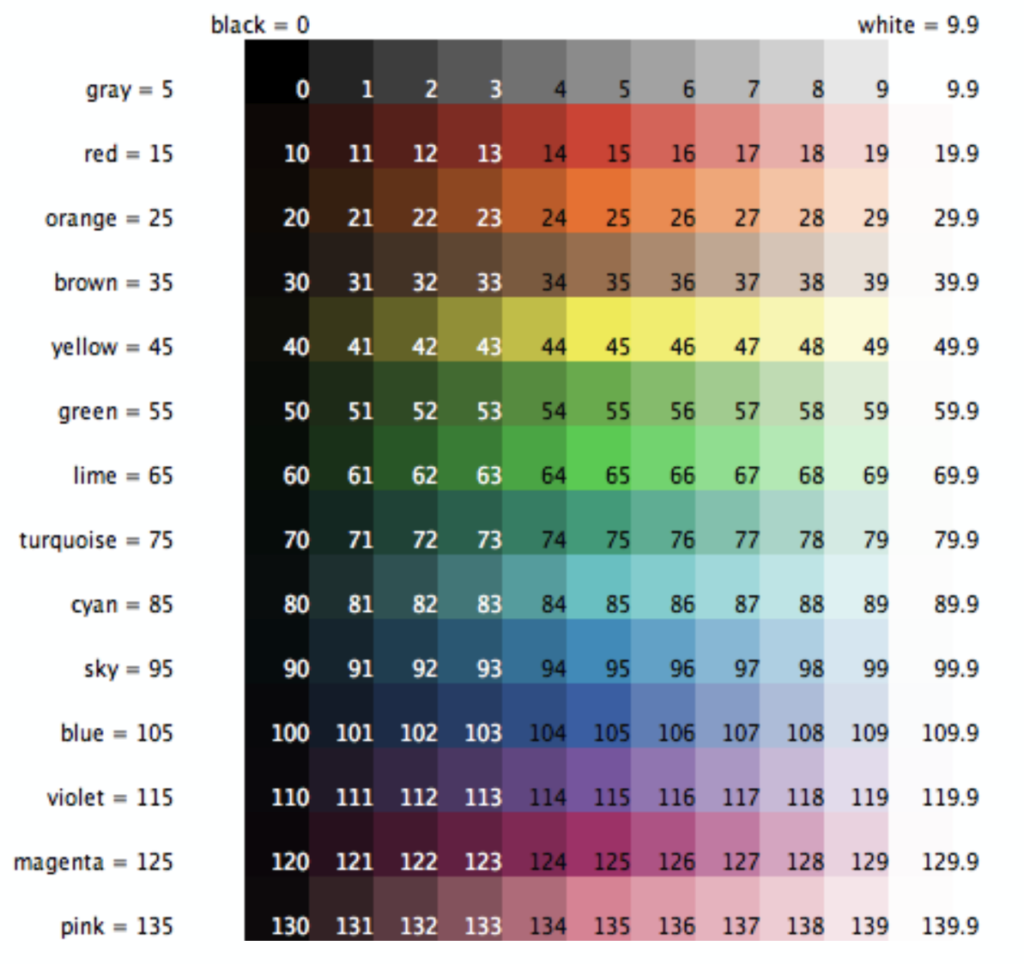
The plants will have these colors:
- Red, if it likes neutral & dry
- Lime, if it likes neutral & wet
- Sky, if it likes acid & dry
- Violet, if it likes acid & wet
The soils will have these colors:
- Orange, if it is neutral & dry
- Green, if it is neutral & humid
- Cyan, if it is acid & dry
- Magenta, if it is acid & wet
Please note that when the colors are close, it means soil and plant are compatible:
- Red/Orange
- Lime/Green
- Sky/Cyan
- Violet/Magenta
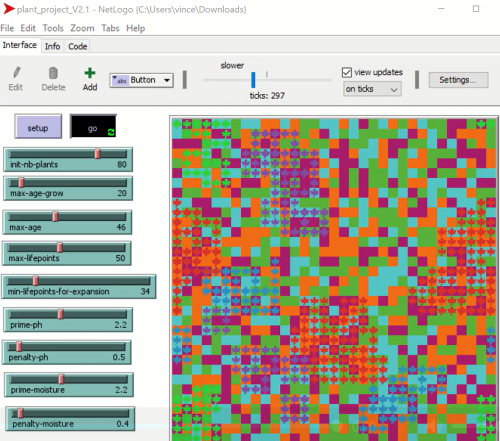
Writing the NetLogo program of the model
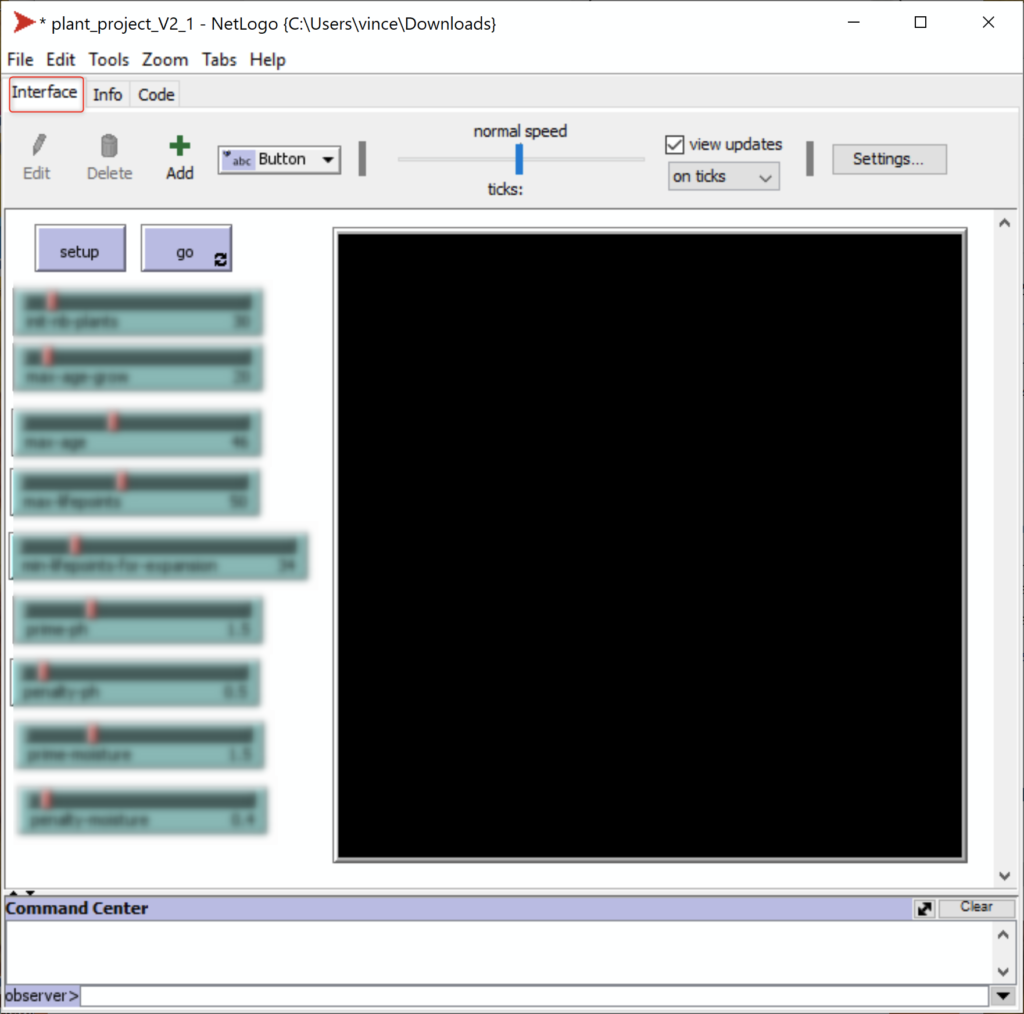
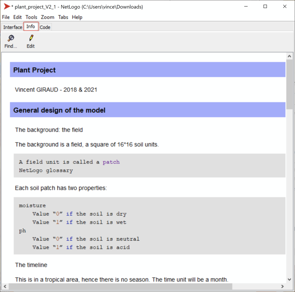
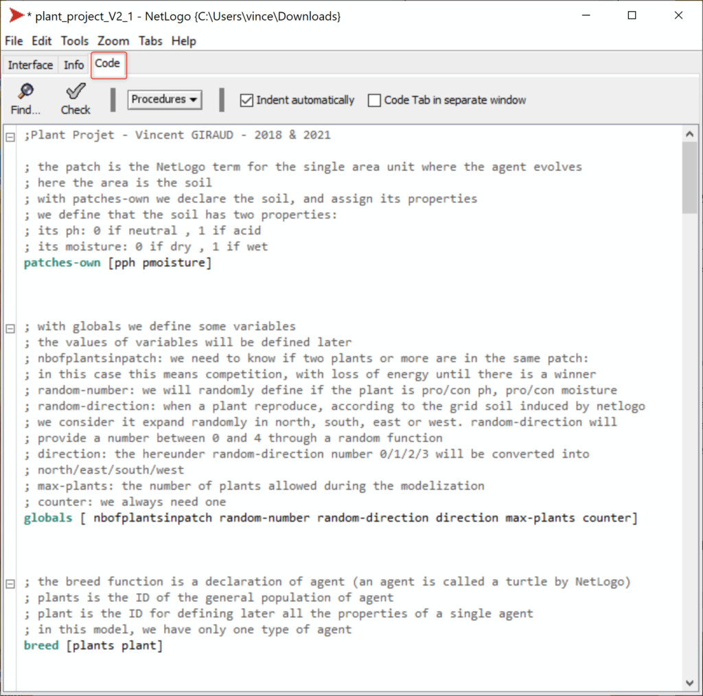
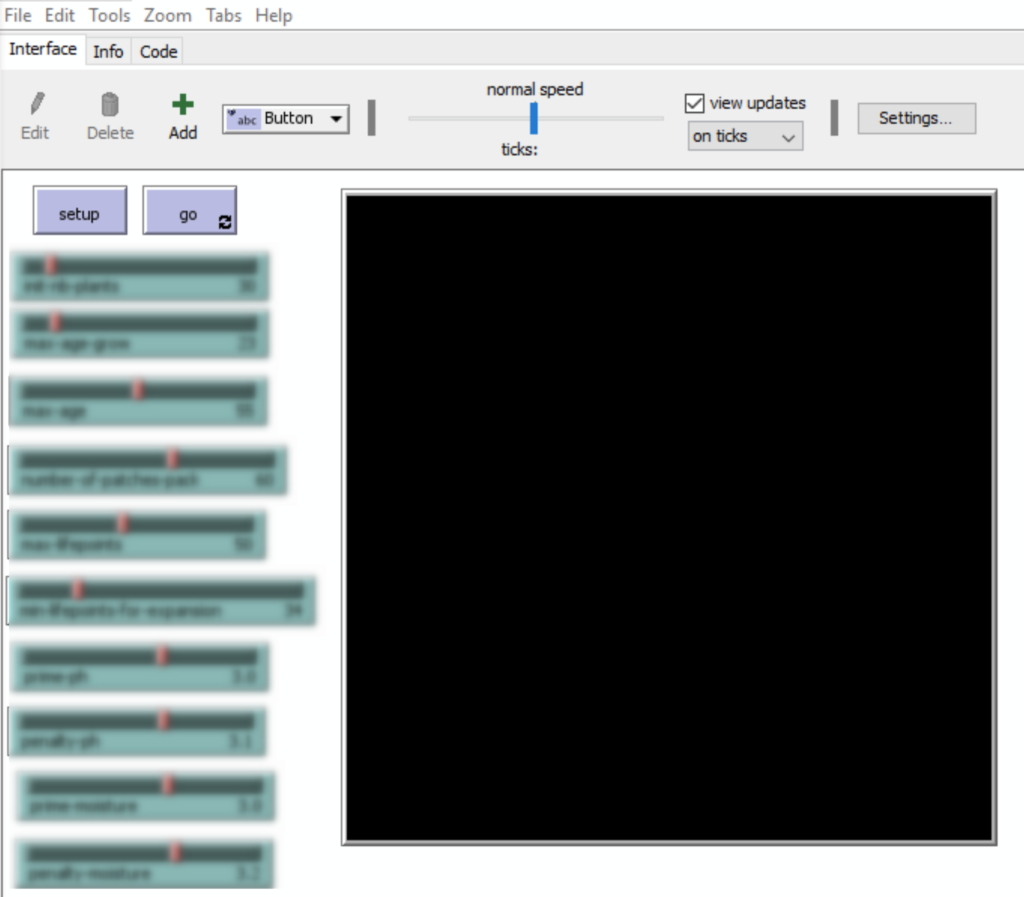
The Netlogo user interface
There are three main windows:
- Interface
- Info
- Code
3 screenshots are provided. They will be detailed later:
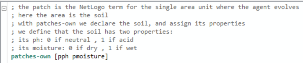
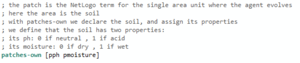
Declaration of the soil
Remark: plant and soil variables can’t have the same name. Hence, the prefix ‘p’ (for the patch) has been added to the patch variable, to ‘ph’ and to ‘moisture’
; the patch is the NetLogo term for the single area unit where the agent evolves
; here the area is the soil
; with patches-own we declare the soil, and assign its properties
; we define that the soil has two properties:
; its ph: 0 if neutral , 1 if acid
; its moisture: 0 if dry , 1 if wet
patches-own [pph pmoisture]
Coding interface
NetLogo has useful coloring functionalities:
In turquoise, there are some main functionalities like declarations and procedures.
In blue: main instructions…
In violet, there are keys like properties of instructions, math functions, and variables.
In red: non-variable values
Management of the field
In the main menu of NetLogo, the size of the soil is defaulted as a 16*16 square and could be changed:
Right-click on the square and choose « edit »:

You can guess the different functionalities.
You can also define that the up border links magically to the down border and that the left border magically links to the right border:

For this program, we keep the initialization parameters as-is.
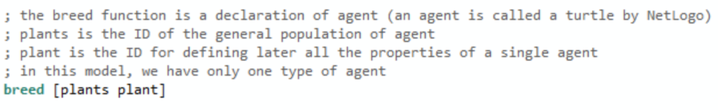
Declaration of the plant agents
; the breed function is a declaration of agent (an agent is called a turtle by NetLogo)
; plants is the ID of the general population of agent
; plant is the ID for defining later all the properties of a single agent
; in this model, we have only one type of agent
breed [plants plant]
Declaration of variables
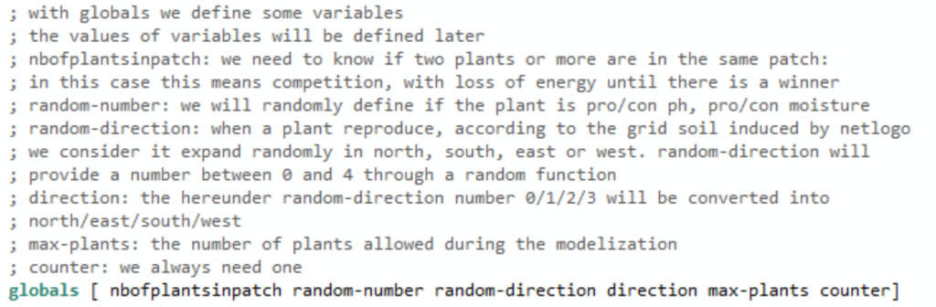
 ; with globals we define some variables
 ; the values of variables will be defined later
; nbofplantsinpatch: we need to know if two plants or more are in the same patch:
 ; in this case this means competition, with loss of energy until there is a winner
; random-number: we will randomly define if the plant is pro/con ph, pro/con moisture
; random-direction: when a plant reproduce, according to the grid soil induced by netlogo
 ; we consider it expand randomly in north, south, east or west. random-direction will
 ; provide a number between 0 and 4 through a random function
 ; direction: the hereunder random-direction number 0/1/2/3 will be converted into
 ; north/east/south/west
; max-plants: the number of plants allowed during the modelization
; counter: we always need one
globals [ nbofplantsinpatch random-number random-direction direction max-plants counter]
Declaration of the initialization parameters
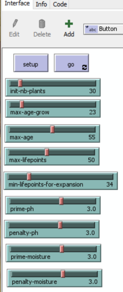
This is done in the « interface » menu:
The following variables are defined:
| Variable | Description | Min | Increment | Max | Default Value |
| init-nb-plants | How many plants are at the start of the model? | 20 | 1 | 100 | 30 |
| max-age-grow | Until which age does the plant naturally gain life points? | 10 | 1 | 100 | 23 |
| max-age | What is the maximum possible age of the plant? | 10 | 1 | 100 | 55 |
| max-lifepoints | What is the maximum number of life points of a plant? | 10 | 1 | 100 | 50 |
| min-lifepoints-for-expansion | What is the number of life points required for a plant for expansion? | 17 | 1 | 100 | 34 |
| prime-ph | What is the life points’ prime if a plant is on ph-compatible soil? | 0 | 0.1 | 5 | 3 |
| penalty-ph | What is the life points penalty if a plant is on moisture-incompatible soil? | 0 | 0.1 | 5 | 3 |
| prime-moisture | What is the life points’ prime if a plant is on moisture-compatible soil? | 0 | 0.1 | 5 | 3 |
| penalty-moisture | What is the life points’ penalty if a plant is on moisture-incompatible soil? | 0 | 0.1 | 5 | 3 |
The result:
Declaration of the plants: their single and plural names
; the breed function is a declaration of agent (an agent is called a turtle by NetLogo)
; plants is the ID of the general population of agent
; plant is the ID for defining later all the properties of a single agent
; in this model, we have only one type of agent
breed [plants plant]
Declaration of the plants: their properties
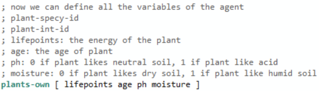
; now we can define all the variables of the agent
; plant-specy-id
; plant-int-id
; lifepoints: the energy of the plant
; age: the age of plant
; ph: 0 if plant likes neutral soil, 1 if plant like acid
; moisture: 0 if plant likes dry soil, 1 if plant like humid soil
plants-own [ lifepoints age ph moisture ]
Setup of the model: initializing the first tick.
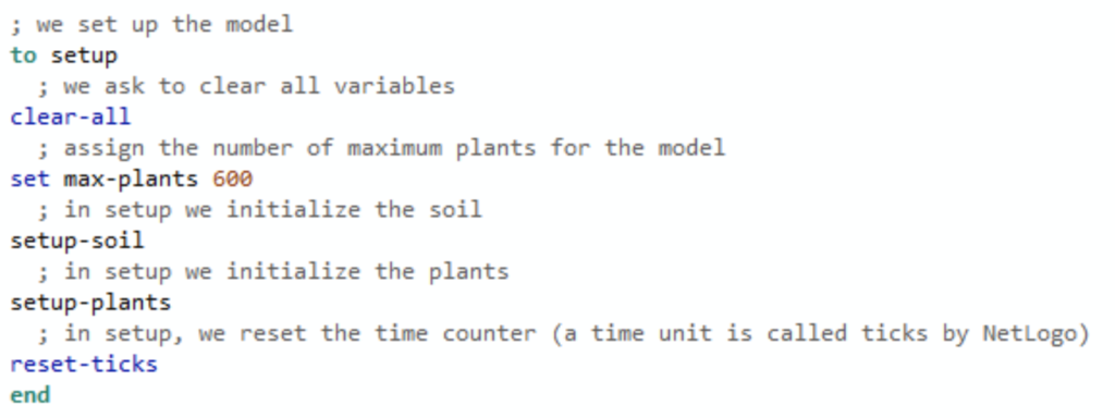
; we set up the model
to setup
  ; we ask to clear all variables
clear-all
  ; assign the number of maximum plants for the model
set max-plants 600
  ; in setup we initialize the soil
setup-soil
  ; in setup we initialize the plants
setup-plants
  ; in setup, we reset the time counter (a time unit is called ticks by NetLogo)
reset-ticks
end
Focus on set-soil
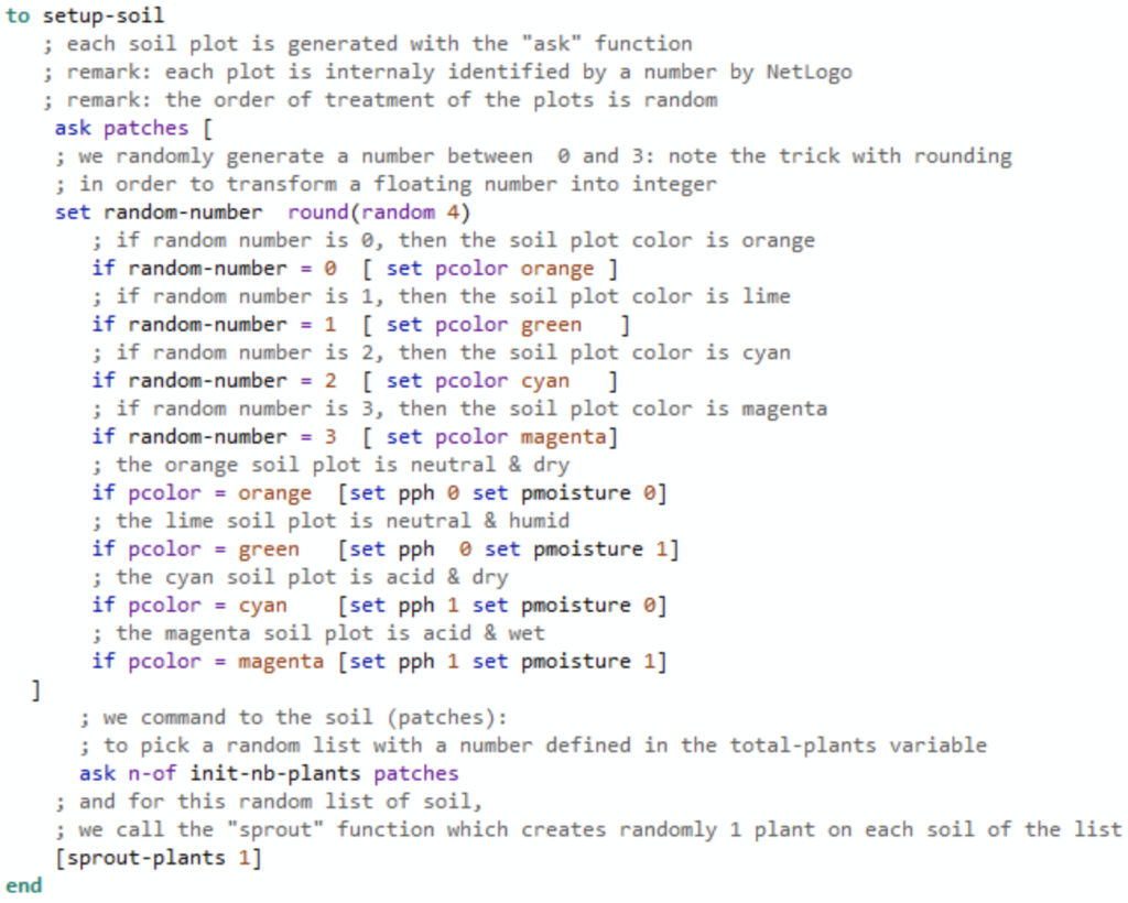
to setup-soil
   ; each soil plot is generated with the "ask" function
   ; remark: each plot is internaly identified by a number by NetLogo
   ; remark: the order of treatment of the plots is random
    ask patches [
    ; we randomly generate a number between  0 and 3: note the trick with rounding
    ; in order to transform a floating number into integer
    set random-number  round(random 4)
       ; if random number is 0, then the soil plot color is orange
       if random-number = 0  [ set pcolor orange ]
       ; if random number is 1, then the soil plot color is lime
       if random-number = 1  [ set pcolor green   ]
       ; if random number is 2, then the soil plot color is cyan
       if random-number = 2  [ set pcolor cyan   ]
       ; if random number is 3, then the soil plot color is magenta
       if random-number = 3  [ set pcolor magenta]
       ; the orange soil plot is neutral & dry
       if pcolor = orange  [set pph 0 set pmoisture 0]
       ; the lime soil plot is neutral & humid
       if pcolor = green   [set pph  0 set pmoisture 1]
       ; the cyan soil plot is acid & dry
       if pcolor = cyan    [set pph 1 set pmoisture 0]
       ; the magenta soil plot is acid & wet
       if pcolor = magenta [set pph 1 set pmoisture 1]
  ]
      ; we command to the soil (patches):
      ; to pick a random list with a number defined in the total-plants variable
      ask n-of init-nb-plants patches
    ; and for this random list of soil,
    ; we call the "sprout" function which creates randomly 1 plant on each soil of the list
    [sprout-plants 1]
end
Focus on setup-plant
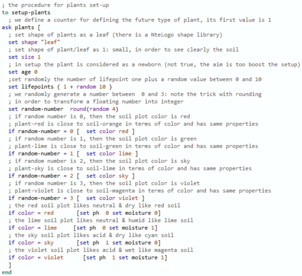
; the procedure for plants set-up
to setup-plants
  ; we define a counter for defining the future type of plant, its first value is 1
ask plants [
  ; set shape of plants as a leaf (there is a NteLogo shape library)
  set shape "leaf"
  ; set shape of plant/leaf as 1: small, in order to see clearly the soil
  set size 1
  ; in setup the plant is considered as a newborn (not true, the aim is too boost the setup)
  set age 0
  ;set randomly the number of lifepoint one plus a random value between 0 and 10
  set lifepoints ( 1 + random 10 )
  ; we randomly generate a number between  0 and 3: note the trick with rounding
  ; in order to transform a floating number into integer
  set random-number  round(random 4)
  ; if random number is 0, then the soil plot color is red
  ; plant-red is close to soil-orange in terms of color and has same properties
  if random-number = 0 [  set color red ]
  ; if random number is 1, then the soil plot color is green
  ; plant-lime is close to soil-green in terms of color and has same properties
  if random-number = 1 [  set color lime ]
  ; if random number is 2, then the soil plot color is sky
  ; plant-sky is close to soil-lime in terms of color and has same properties
  if random-number = 2 [  set color sky ]
  ; if random number is 3, then the soil plot color is violet
  ; plant-violet is close to soil-magenta in terms of color and has same properties
  if random-number = 3 [  set color violet ]
  ; the red soil plot likes neutral & dry like red soil
  if color = red       [set ph  0 set moisture 0]
  ; the lime soil plot likes neutral & humid like lime soil
  if color = lime     [set ph  0 set moisture 1]
  ; the sky soil plot likes acid & dry like cyan soil
  if color = sky       [set ph  1 set moisture 0]
  ; the violet soil plot likes acid & wet like magenta soil
  if color = violet      [set ph  1 set moisture 1]
  ]
end
Management of each month’s cycle
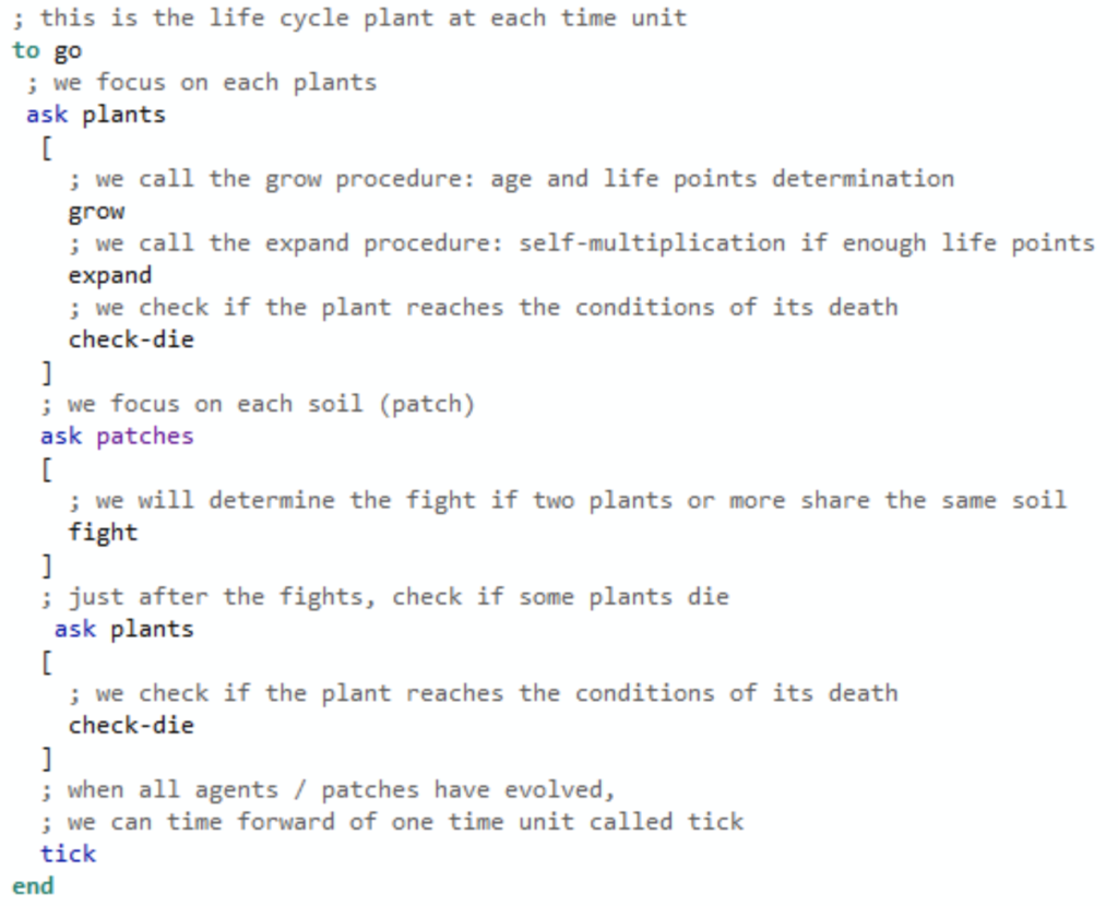
; this is the life cycle plant at each time unit
to go
 ; we focus on each plants
 ask plants
  [
    ; we call the grow procedure: age and life points determination
    grow
 ; this is the life cycle plant at each time unit
to go
 ; we focus on each plants
 ask plants
  [
    ; we call the grow procedure: age and life points determination
    grow
    ; we call the expand procedure: self-multiplication if enough life points
    expand
    ; we check if the plant reaches the conditions of its death
    check-die
  ]
  ; we focus on each soil (patch)
  ask patches
  [
    ; we will determine the fight if two plants or more share the same soil
    fight
  ]
  ; just after the fights, check if some plants die
   ask plants
  [
    ; we check if the plant reaches the conditions of its death
    check-die
  ]
  ; when all agents / patches have evolved,
  ; we can time forward of one time unit called tick
  tick
end
The plant growth
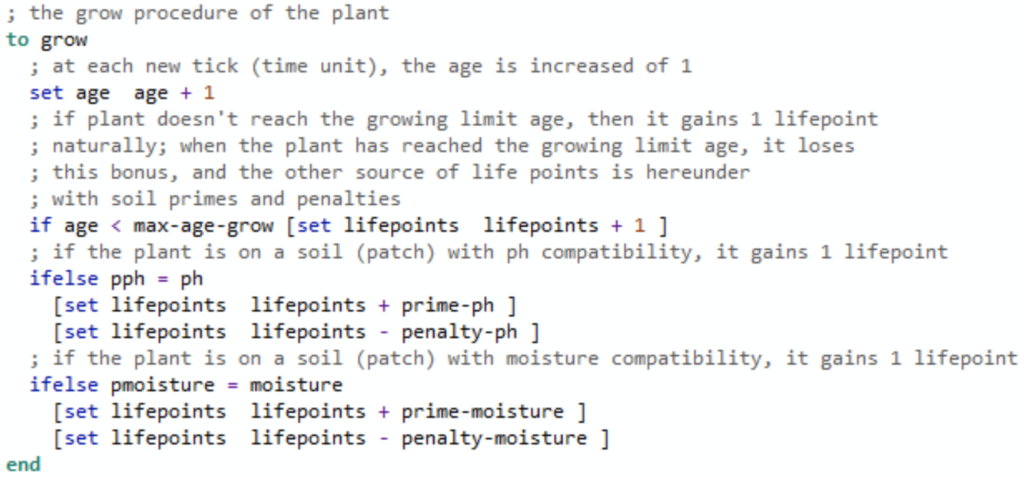
; the grow procedure of the plant
to grow
  ; at each new tick (time unit), the age is increased of 1
  set age  age + 1
  ; if plant doesn't reach the growing limit age, then it gains 1 lifepoint
  ; naturally; when the plant has reached the growing limit age, it loses
  ; this bonus, and the other source of life points is hereunder
  ; with soil primes and penalties
  if age < max-age-grow [set lifepoints  lifepoints + 1 ]
  ; if the plant is on a soil (patch) with ph compatibility, it gains 1 lifepoint
  ifelse pph = ph
    [set lifepoints  lifepoints + prime-ph ]
    [set lifepoints  lifepoints - penalty-ph ]
  ; if the plant is on a soil (patch) with moisture compatibility, it gains 1 lifepoint
  ifelse pmoisture = moisture
    [set lifepoints  lifepoints + prime-moisture ]
    [set lifepoints  lifepoints - penalty-moisture ]
end
The plant may die
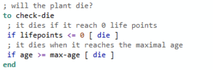
; will the plant die?
to check-die
 ; it dies if it reach 0 life points
 if lifepoints <= 0 [ die ]
 ; it dies when it reaches the maximal age
 if age >= max-age [ die ]
end
The plant expansion
; does the plant expand / create 8 new sowings?
; procedure "expand"
to expand
  ; check if the life points is greater than
  ; the minimum life points for expansion
  if lifepoints > min-lifepoints-for-expansion
  [
    ; if yes, the plant loses 16 life points, and
    ; they are transfered to its 8 new sowings:
    ; 2 life points for each new sowing
    set lifepoints  lifepoints - 16
    ; we call 8 times the procedure that creates sowing
    ; we need a counter:
    ; first at zero value, it's the north direction
    ; then it will become 45, 90, 135, 180, 225, 270, 315
    ; meaning: north-east, east, south-east, south, south-west, west, north-west
set counter  0
    repeat 8 [
      ; call the procedure creating new sowing with the direction as input parameter
      new-sowing counter
      ; rotate the direction
      set counter counter + 45
             ]
  ]
end
The details of the creation procedure
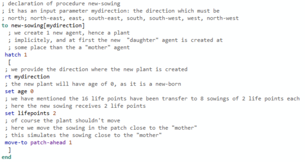
; declaration of procedure new-sowing
; it has an input parameter mydirection: the direction which must be
; north; north-east, east, south-east, south, south-west, west, north-west
to new-sowing[mydirection]
  ; we create 1 new agent, hence a plant
  ; implicitely, and at first the new  "daughter" agent is created at
  ; some place than the a "mother" agent
 hatch 1
  [
 ; we provide the direction where the new plant is created
 rt mydirection
 ; the new plant will have age of 0, as it is a new-born
 set age 0
 ; we have mentioned the 16 life points have been transfer to 8 sowings of 2 life points each
 ; here the new sowing receives 2 life points
 set lifepoints 2
 ; of course the plant shouldn't move
 ; here we move the sowing in the patch close to the "mother"
 ; this simulates the sowing close to the "mother"
 move-to patch-ahead 1
  ]
end
The plant fight
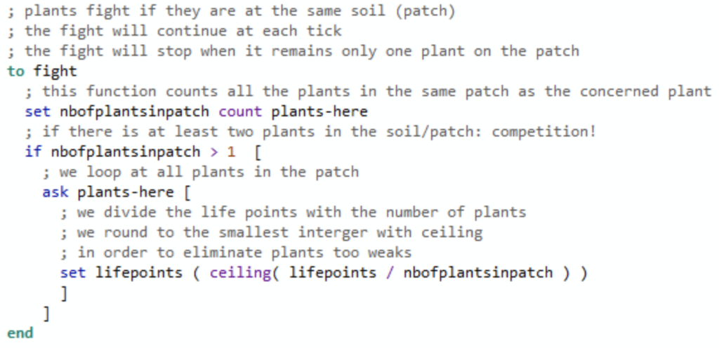
If two plants or more are at the same patch, they will fight and lose life points. In the end, there can be only one.
; plants fight if they are at the same soil (patch)
; the fight will continue at each tick
; the fight will stop when it remains only one plant on the patch
to fight
  ; this function counts all the plants in the same patch as the concerned plant
  set nbofplantsinpatch count plants-here
  ; if there is at least two plants in the soil/patch: competition!
  if nbofplantsinpatch > 1  [
    ; we loop at all plants in the patch
    ask plants-here [
      ; we divide the life points with the number of plants
      ; we round to the smallest interger with ceiling
      ; in order to eliminate plants too weaks
      set lifepoints ( ceiling( lifepoints / nbofplantsinpatch ) )
      ]
    ]
end
The downloadable content
This is the file with .nlogo format:
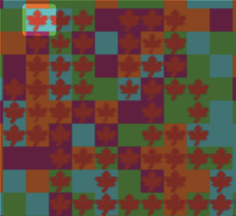
Simulation of the Plant 4-Species Competition
Hereunder is a video simulation:
Few tips about Netlogo programming
Feel free to fast-forward or slow-forward for analysis:

Feel free to inspect individually the plants and the patches:
Right-click on a patch:
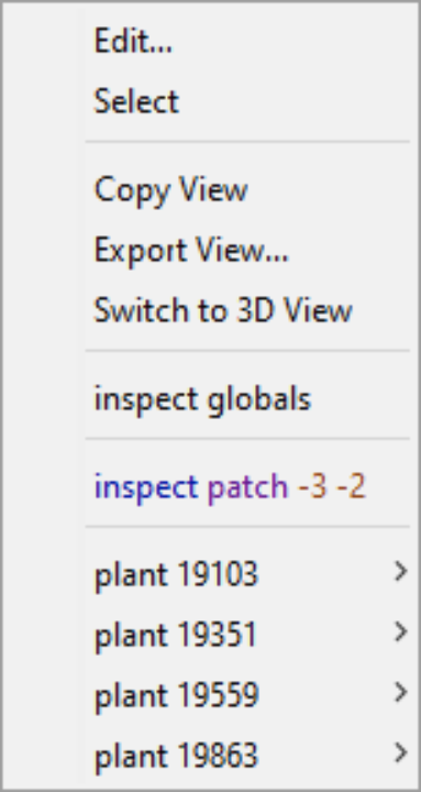
You can get details about the patch and the plants on it.
An inconvenient: it is not obvious if there are two plants or more on the same patch
Hence, the inspection will help:

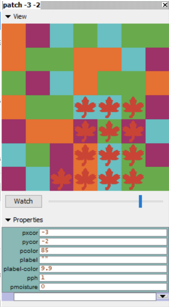
For example, inspection of the patch by clicking on

A new window is opened with properties like ph (pph) and moisture (pmoisture):
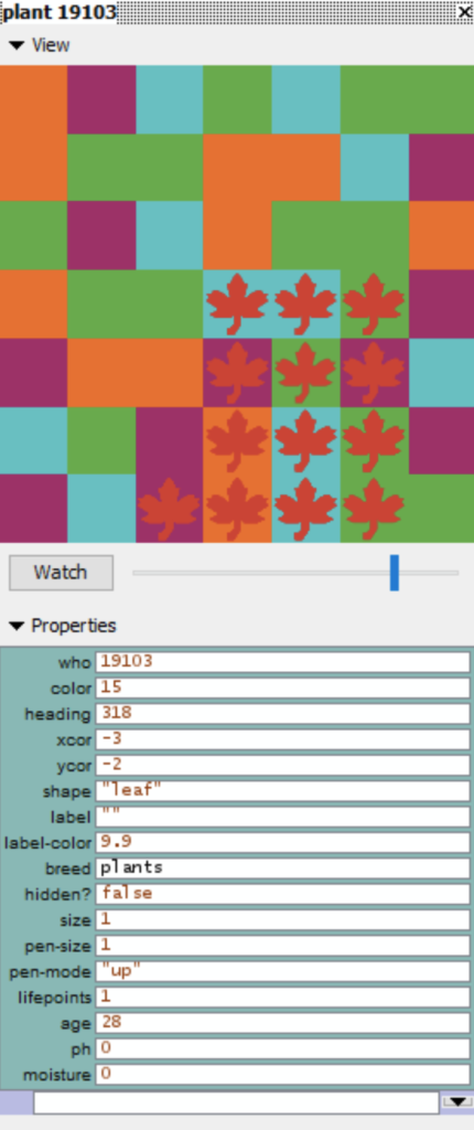
Three actions are possible for each plant:
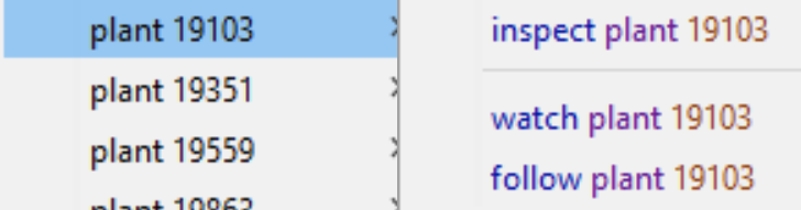
« Inspect » opens a new window with all the properties:
« Watch » creates a visual focus:

Follow creates a more discrete visual focus:

Conclusion
NetLogo is the perfect tool for understanding and developing Agent-Based Models (ABM).
With the own-developed Plant 4-Species Competition model, we have detailed how an ABM project could be developed.
- We have seen how the agents (plants) and their backgrounds (patches) are managed.
- Also, the evolution of the agents (grow, die, expand), the agents/agents interactions (fight), and the agent/background interaction (prime and penalty of soil compatibility) have been taken into account and developed.
This deep dive has helped us understand how to develop an Agent-based model.