A* is pronounced « A star »
Prerequisite
The knowledge of the Dijkstra algorithm is required:
A* algorithm in short
Just remember its properties:
- It’s methodical: it will, without doubt, find the shortest path
- It is a variant of the Dijkstra algorithm:
- With Dijkstra, the actual distances from the source to the intermediary nodes are calculated, and there is no clue about the distances from the intermediary nodes to the destinations. The minimum distance is chosen first.
- With A*, the actual distances from the source to the intermediary nodes are also calculated and added to the estimated distances from the intermediary nodes to the destinations.
- It’s not hard to apply
A* often applies for finding a solution, not mandatorily the shortest one: in this scenario, the search is stopped as soon as the first solution is found.
It’s why it is usually designated as a search algorithm.
And it is too a shortest path algorithm with the scenario « searching all solutions ».
Context with a TSP example
This is the same example as in the Dijkstra article, in order to compare
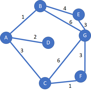
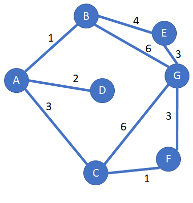
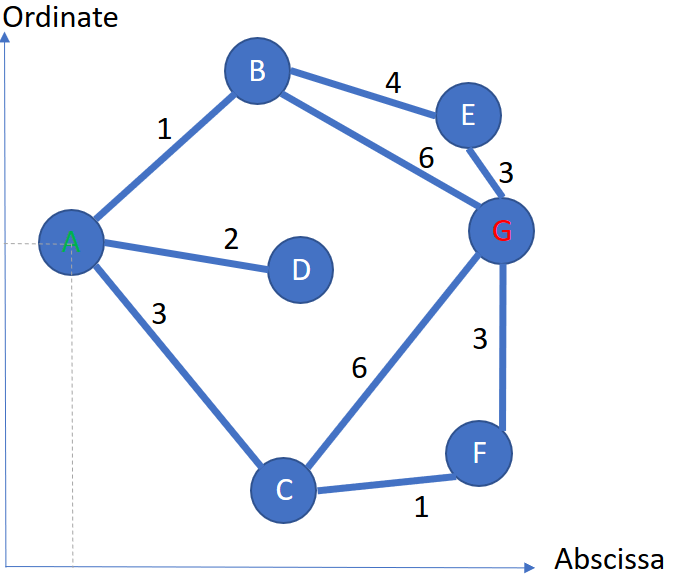
Imagine you want to travel from city A to city G.
Your aim is to minimize the traveling time, which is counted with unit « hour ».
You are traveling with the railroad. The time is not fully linked to the distance: some trains are high-speed/mid-speed/low-speed. Between cities, it may be plain/hill/mountain land.
Each city is networked to a limited number of other cities
What’s the shortest time for traveling from A to G? Which is the best according to
Why and how to estimate distances from intermediary nodes to the target node?
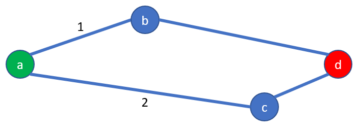
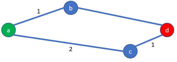
Let’s have a look at this example: the problem is to find the shortest path between the cities (a) and (d), and the distances will be revealed step by step in order not to spoil the explanation:
Application of Dijkstra
With Dijkstra, applying the first step will provide these distances, and the shortest distance starting from (a) is the city (b).
As (b) is closer to (a) than (c
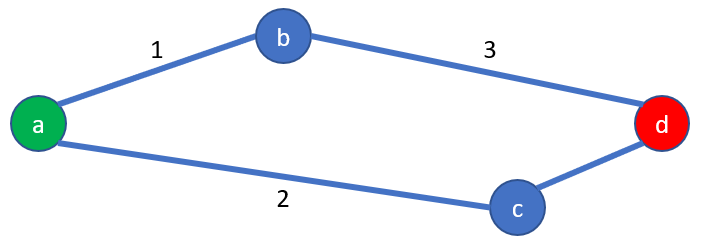
Then it remains to calculate the distances starting from (d): the total distance between (a) -> (c) -> (d) is 3 hours
The shortest path is (a) -> (c) -> (d) with a distance of 3 hours
Estimation of distances with A*
Like with a map, we will estimate the distance between 2 cities as the distance in centimeters.

On my own screen, the distance between (b) and (d) is around 9 cm, and the distance between (c) and (d) is around 3 cm.
Applying a scale like in any roadmap, I have arbitrarily defined 3cm is equal to a distance of 1 hour.
Hence the distance between:
- (b) and (d) is 3 hours estimated
- (c) and (d) is 1 hour estimated
Application of A*
With A*, we are starting too from (a), and (b) + (c) are its neighbor cities:
Please remember (b) -> (d) and (c) -> (d) are not yet known
A* is estimating the distances between (a) and (d), through (b) and (d) like this:
- Distance (a) -> (b) -> (d) is calculated as sum of the known (a) -> (b) 1 hour and estimation of (b) -> (d) 3 hours, hence the partially estimated total is 4 hours
- Distance (a) -> (c) -> (d) is calculated as sum of the known (a) -> (c) 2 hours and estimation of (c) -> (b) 3 hours, hence the partially estimated total is 4 hours
Hence, the travel (a) -> (c) -> (d) must be calculated before the (a) -> (b) -> (d), because it seems promising
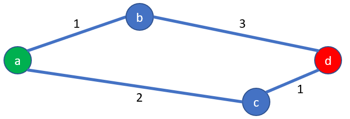
When considering the travel (a) -> (c) -> (d) : the distance (c) -> (d) can be revealed, and the real total distance, without estimation, is 3 hours.
In conclusion, in this example, A* is finding the shortest path before Dijkstra, thanks to the estimation of the distance remaining between the intermediate city and the target city.
The estimation is called heuristic in the A* litterature.
A heuristic technique (/hjʊəˈrɪstɪk/; Ancient Greek: εὑρίσκω, « find » or « discover »), or a heuristic for short, is any approach to problem solving or self-discovery that employs a practical method that is not guaranteed to be optimal, perfect or rational, but which is nevertheless sufficient for reaching an immediate, short-term goal https://en.wikipedia.org/wiki/Heuristic
Estimation/heuristic: example and limitations
Unsurprisingly, the estimation depends on your knowledge or of your data.
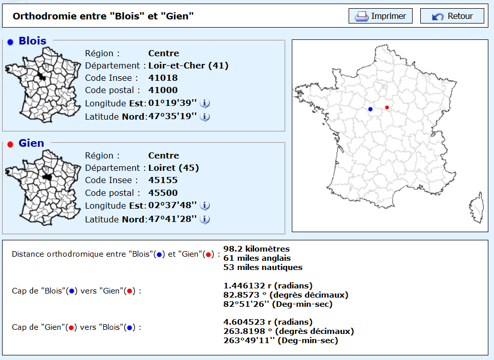
We illustrate this with a map example: the estimated travel by car from Gien to Blois, both of which are French cities.
Scenario 0:
Above, we note there is no sufficient estimation of the distance between Blois and Gien: forget A*, and choose the Dijkstra algorithm:
Scenario 1:
If you don’t know the road network, you could fetch the GPS. Considering arbitrarily a mean speed of 60 km/h, it is converted into hours, and the result is 98.2/60 ≃ 1.64 hours ≃ 1 hour 38 minutes.
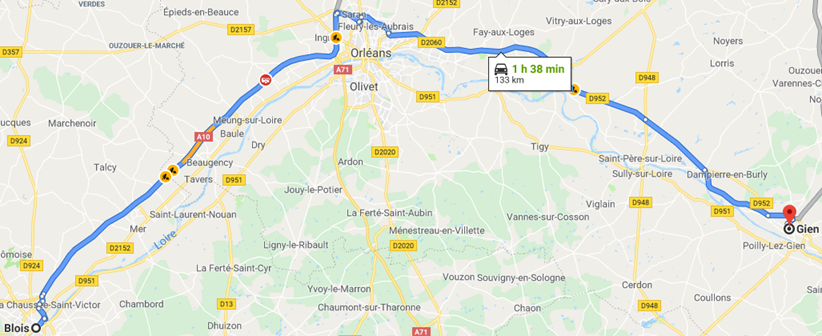
Scenario 2:
If you don’t know the existence of the highway, the estimated distance is 1h49min.

Scenario 3:
If you have the entire road network knowledge, the estimated distance is 1h38, thanks to the highway.
Disclaimer:
An estimation might be fully wrong: for instance, there is no road between Jersey and Guernesey, nevertheless, the coordinates would indicate a value of around 30 kilometers.
A* might deal with estimation big mistakes.
Applying A* step by step
The shortest path to solve
Imagine you want to travel from city A to city G:
Preparation of the solving tool
First, let’s create a table which will store our step-by-step process:
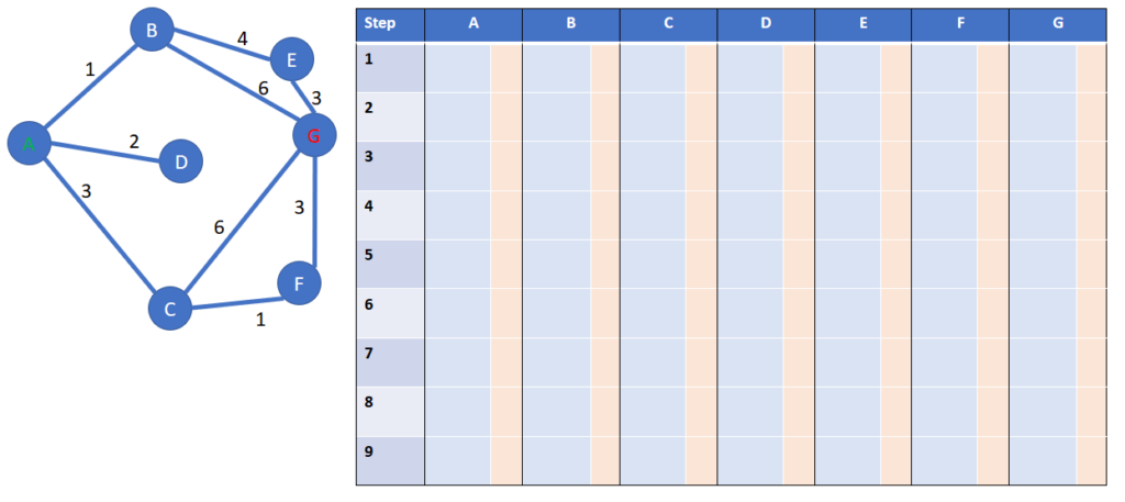
The rows of this table: at each new step we will focus on a new “milestone” city, start a new row and do some calculations

The columns of this table: each existing city receives 2 sub-columns:
- In the light blue background sub-cell: the distance in hours
from the start of city A to the city corresponding to the city owning this
column - In the light orange background sub-cell the previous city of the path, that has lead to the city owning this column

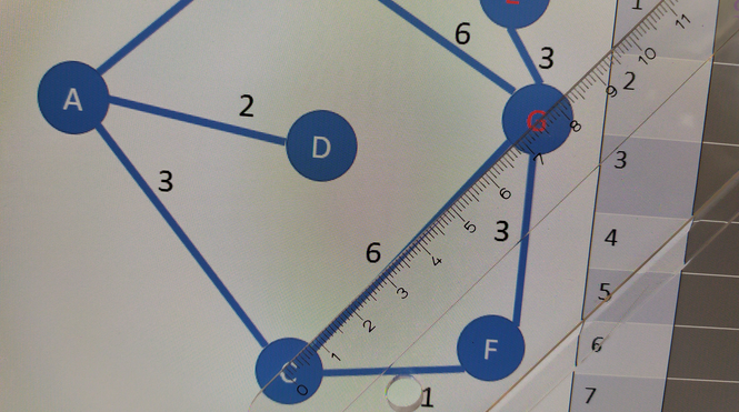
Remark: how to estimate the distances in our example?
I’m measuring the estimated distances on my own screen. And I have arbitrarily chosen 1 cm = 1 hour. It means your distances will be different on your screen.
Here the estimated distance between city B and G is 7.4 cm meaning 7.4 hours.
The following estimated distances will include bold font value.
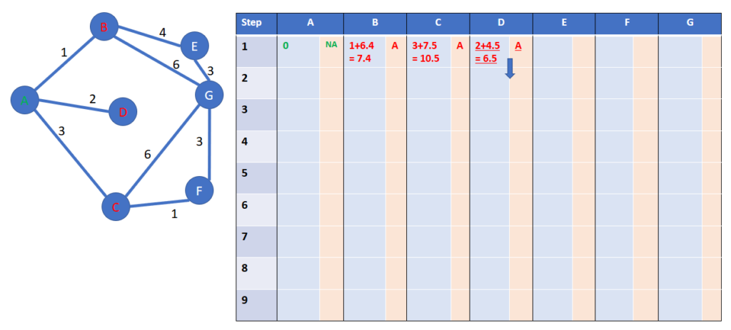
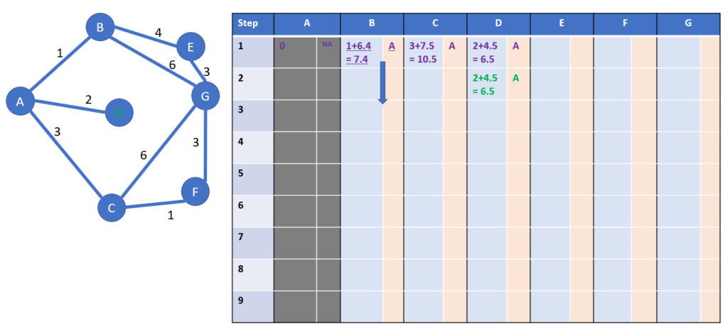
Step 1: starting from city A
This step is special, we fill the cell A1 in green font with:
- The distance is equal to 0, as the path from A to A is null
- The previous city is NA for “Not Applicable”: A is the starting city, hence it has no previous city
- We grey column A at the end of this step: we won’t come back to A, as it would mean a waste of distance, hereunder is a small example of why coming again to city A would be a loss of time
Now we check which cities are linked to A: there are B, C, D
We calculate the 3 distances from A to G through B, C, D:
- Real distance from A to B + estimated distance from B to G = 1 + 6.4 = 7.4 hours
- Distance from A to C + estimated distance from C to G = 3 + 7.5 = 10.5 hours
- Distance from to D + estimated distance from D to G: 2 + 4.5 = 6.5 hours
The non-grey column with the minimum total distance, including estimation, is the one for city D: it is copied to the next row; see the blue arrow.
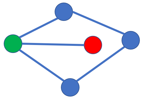
In the left figure: Starting from green city, no need to travel the blue loop before reaching the red city: it’s why we don’t come back to a previous city
Step 2: starting from D
We will grey the column D at the end of the step: we won’t come back to D, as it would mean a waste of distance
Now we check which cities are linked to D: the answer is no one!
Yes, this is a dead way. Indeed I had included it in order to show an example of an estimation pitfall. When you guess, you can have [perfect/correct/far away/totally wrong] result.
The non-grey column with the minimum total distance including estimation is the one of city B: it is copied to the next row, see the blue arrow.
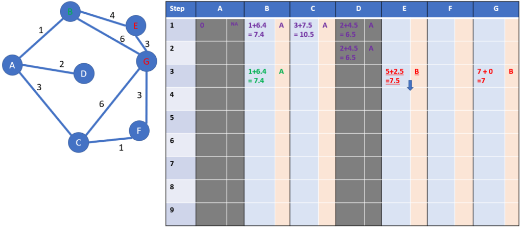
Step 3: starting from B
We will grey the column B at the end of the step: we won’t come back to B, as it would mean a waste of distance
Now we check which cities are linked to B: the answer is E and G.
We calculate the distances from A to G through B, and then through E and G (as G is the destination, no need for estimation):
- Real distance from A to B + estimated distance from B to G = (1 + 4) + 2.5 = 7.5 hours
- Distance from A to G fully calculated= (1+6) = 7 hours
We have the first solution from A to G; we are curious if it is the shortest.
The non-grey column with the minimum total distance including estimation is the one of the city E: it is copied to the next row, see the blue arrow.
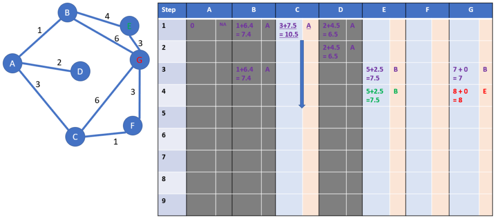
Step 4: starting from E
We will grey the column E at the end of the step: we won’t come back to E, as it would mean a waste of distance
Now we check which cities are linked to B: the answer is only G.
We calculate the distance from A to G through E. As G is the destination, no need for estimation):
- Distance from A to G through E fully calculated= (1+4+3) = 8 hours
We have the second solution from A to G. Please keep in mind we will check only at the end of the algorithm if it is the shortest.
The non-grey column with the minimum total distance including estimation is the one of the city C: it is copied to the next row, see the blue arrow.
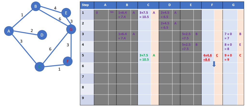
Step 5: starting from C
We will grey the column C at the end of the step: we won’t come back to C, as it would mean a waste of distance
Now we check which cities are linked to B: the answers are F and G.
We calculate the distance from A to G through F and G.
- Distance from A to G through F calculated and estimated = (3+6) = 9 hours
- Distance from A to G « through G » indeed is fully calculated = (3+1)+4.6 = 8.6 hours
We have the third solution from A to G. Please keep in mind we will check only at the end of the algorithm if it is the shortest.
The non-grey column with the minimum total distance, including estimation, is the one for city F: it is copied to the next row; see the blue arrow.
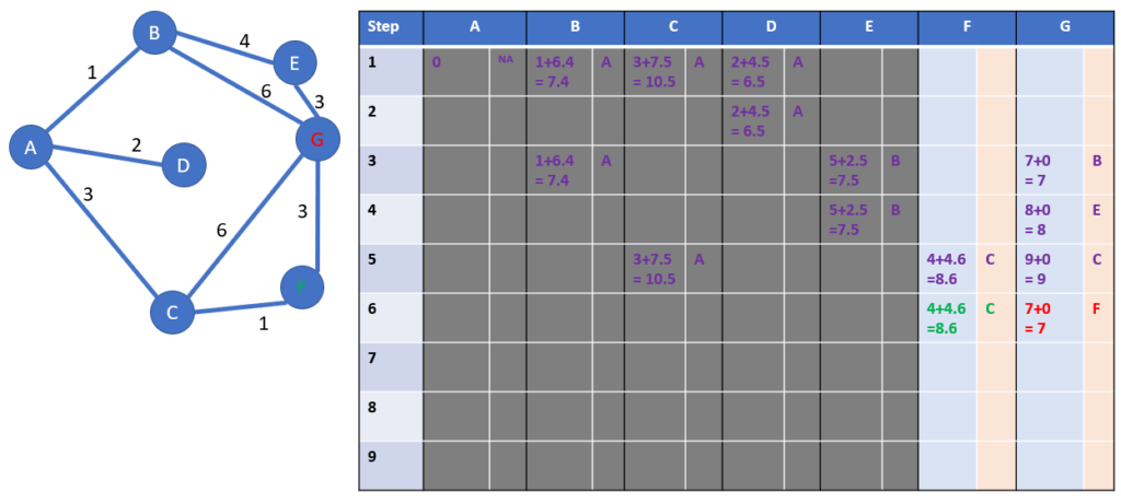
Step 6: starting from F
We will grey the column F at the end of the step: we won’t come back to F, as it would mean a waste of distance
Now we check which cities are linked to F: the answer is G.
We calculate the distance from A to G through F.
- Distance from A to G « through G » indeed is fully calculated = (3+1+3) = 7 hours
We have the fourth solution from A to G. Please keep in mind we will check only at the end of the algorithm if it is the shortest.
The non-grey column with the minimum total distance including estimation is the one of the city G: let’s read the meters in the next step
Step 6: what is the shortest distance?
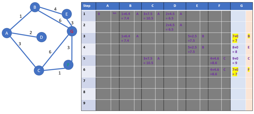
There are 2 winners with a distance from A to G of 7 hours.
Step 7: what is the shortest path?
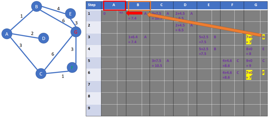
We choose arbitrarily one of the winners, the one with B as the predecessor. Column per column, we can trace back the path:
- As arbitrarily chosen, from G to B, thanks to the orange arrow, finding back the right column with the orange box
- Then from B to A, thanks to the red arrow, finding back the right column with the red box
The reversed path is G -> B -> A
We reverse the reversed path, and we get one of the two solutions A -> B -> G
Algorithm description
We have started with a concrete example, we are ready to become more abstract: let’s describe the algorithm, as it could become the specification of a program, whatever the language
We start with the definition of the variants. There are three kinds of tables:
- Unvisited cities: the cities which we have not yet studied the paths with this city, current, visited)
- Current city: the milestone city from which we are investigating the nieghbor paths
- Visited cities: the cities in which we have already calculated the paths
The columns will be explained just after this step.
Creation of variables
First we need a variable table in order to store the unvisited cities :
| City |
| … |
| … |
| … |
Then a second variable table in order to store the current city:
| City | Distance from starting city | Previous City |
| … | … | … |
| … | … | … |
| … | … | … |
Then a third variable table in order to store the visited cities
| City | Distance from starting city | Previous City |
| … | … | … |
| … | … | … |
| … | … | … |
The algorithm in shortest path configuration
- List all cities and store them in the unvisited table, column City
- Is it the first time in this step?
- If yes, select city “starting city”
- If no, select the city from the visited table with the smallest distance AND with its corresponding City which is not in the unvisited table.
- The city from step 2 is removed from the unvisited table
- Look for all neighboring cities in the city from step 2. Create a row in the current table for each of these neighbors. Is it the first time this step has been taken?
- If yes:
- The city is “starting city”
- Distance is “0”
- Previous city is “NA”
- If no :
- The city is “the considered neighbor”
- Total distance is the sum of the distance from “starting city” to “city selected in step 2” (keep in mind it has already been calculated and stored in the visited table) + estimated distance from “city selected in step 2” to “the target”
- The previous city is “city selected in step 2”
- If yes:
- Move the row(s) from the current table to the visited table
- Is the unvisited table empty?
- If yes: go to step 7
- If no: repeat steps 2 to 6
- Find in the visited table the row with City column equal to the destination city, and with the smallest distance value. Get the previous city. Go to the row where the City column is equal to the previous city, and with the smallest distance value. Repeat as many times as needed in order to reach the starting city as the previous city. Sum all successive distances.
Please note the only difference with the Dijkstra is the sub-step in bold from step 4.
The algorithm in search configuration
- List all cities, and store them in the unvisited table, column City
- Is it the first time in this step?
- If yes, select city “starting city”
- If no, select the city from the visited table with the smallest distance AND with its corresponding City which is not in the unvisited table.
- The city from step 2 is removed from the unvisited table
- Look for all neighboring cities in the city from step 2. Create a row in the current table for each of these neighbors. Is it the first time this step has been taken?
- If yes:
- City is “starting city”
- Distance is “0”
- Previous city is “NA”
- If no :
- City is “the considered neighbor”
- Total distance is the sum of distance from “starting city” to “city selected in step 2” (keep in mind it has already been calculated and stored in visited table) + estimated distance from “city selected in step 2” to “the target”
- Previous city is “city selected in step 2”
- If yes:
- Move the row(s) from the current table to the visited table
- Is the target city reached?
- If yes: go to step 7
- If no: repeat steps 2 to 6
- Find in the visited table the row with City column equal to the destination city. Get its Distance. Get the previous city. Go to the row where the City column is equal to the previous city, and with the smallest distance value. Repeat as many times as needed in order to reach the starting city as the previous city.
Please note the only differences with the Dijkstra are in from step 4, and the step 6.
An application with Python
The package networkx has been chosen: https://networkx.github.io/
Preparation
First we call the package, plus one for plotting:
import networkx as nx
import matplotlib.pyplot as plt
Then we translate this graph in a format compatible with networks, with the name mygraph :
mygraph = nx.Graph()
mygraph.add_edge('A', 'B', weight=1)
mygraph.add_edge('A', 'C', weight=3)
mygraph.add_edge('A', 'D', weight=2)
mygraph.add_edge('B', 'E', weight=4)
mygraph.add_edge('B', 'G', weight=6)
mygraph.add_edge('E', 'G', weight=3)
mygraph.add_edge('C', 'F', weight=1)
mygraph.add_edge('C', 'G', weight=6)
mygraph.add_edge('F', 'G', weight=3)
Let’s draw the result, and compare with the initial graph:
nx.draw(mygraph, with_labels=True)
plt.show()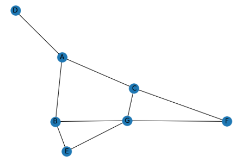
For my information, what are the couple of neigbors, the edges?
for edge in mygraph.edges():
    print(edge)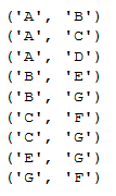
What’s the shortest path between A and G in a Dijkstra configuration? And print it directly.
print(nx.single_source_dijkstra(mygraph,'A','G'))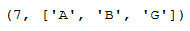
Solving with an A* configuration
Let’s prepare the function that estimates the distances, arbitrarily chosen, as we provide the coordinates with abscissa and ordinate. Then, indicating two cities, the distance as the crow flies can be calculated.
https://en.wikipedia.org/wiki/Cartesian_coordinate_system#Distance_between_two_points
I have printed the initial graph, and then with a graduated scale, I have measured the abscissa and ordinate for each city. For instance, the result was 1.7 as abscissa, and 5.2 as ordinate for city A.
import numpy  # Numpy -> Array manipulation
import pandas # Pandas -> DataFrame : data manipulation

array_coordinates = numpy.array([
    ['A', 1.7, 5.2], # coordinates of city A
    ['B', 4.8, 8.2], # coordinates of city B
    ['C', 5.1, 1.2], # coordinates of city C
    ['D', 5.4, 4.8], # coordinates of city D
    ['E', 8.2, 7.4], # coordinates of city E
    ['F', 8.3, 1.8], # coordinates of city F
    ['G', 8.7, 5.4], # coordinates of city G
])

pandas_coordinates = pandas.DataFrame(array_coordinates, columns = ['CITY', 'X', 'Y'])  # naming the columns

pandas_coordinates.set_index('CITY',inplace=True) # creating the index
How does our coordinate table looks like?
print(pandas_coordinates)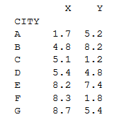
We display the coordinates of city B:
print(pandas_coordinates.loc['B','X'])
print(pandas_coordinates.loc['B','Y'])
We need to convert the coordinates in float format:
pandas_coordinates['X'] = pandas_coordinates['X'].astype(float)
pandas_coordinates['Y'] = pandas_coordinates['Y'].astype(float)
We need to create a python function which estimates the distance between two cities:
def distance_estimation(C1, C2):
    x1 = pandas_coordinates.loc[C1,'X']
    y1 = pandas_coordinates.loc[C1,'Y']
    x2 = pandas_coordinates.loc[C2,'X']
    y2 = pandas_coordinates.loc[C2,'Y']
    return ((x1 - x2) ** 2 + (y1 - y2) ** 2) ** 0.5
For instance, we can check one distance estimation:
distance_estimation('A','B')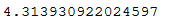
We can include the function in the call of the astar_path function:
nx.astar_path(mygraph, 'A', 'G', distance_estimation)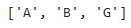
Comparison between A* and Dijkstra
Both provide the shortest path: it usually is an advantage.
If there are too many nodes (or cities), it induces many calculations and this could become a problem for both.
A* often finds a short solution (not necessarily the shortest) quicker than Dijkstra, thanks to estimating the shortest remaining path.
Also, A* can try a lousy solution due to the false, incomplete, or missing information estimation. This Wikipedia example https://commons.wikimedia.org/wiki/File:Weighted_A_star_with_eps_5.gif only estimates distance; it doesn’t include the obstacles. Netherveless, you can see that a workaround for the obstacle has been found rapidly. In the same scenario, Dijkstra would try everything around the starting point.

Hereunder a good video illustration from UNSWMechatronics, in a search configuration: A* almost always is better than Dijkstra.
Conclusion
Except for particular cases, A* is more efficient than Dijkstra.